Introduction to useful functions in Excel
MVEN10 Risk Assessment in Environment and Public Health
Exercise overview
- Work alone on your own laptop
Background
Microsoft Excel is a common software in risk analysis. The primary use is to organise and extract data, but it is also possible to build models and perform analysis and simulations in Microsoft Excel.
There are several commercial add-on packages designed for specific purposes. One example is @RISK for probabilistic risk analysis in Excel. It includes functions such as fitting distributions to data and performing Monte Carlo simulation.
We are not teaching using @RISK at this course, but you are welcome to download a free demo and try it.
Another example is the Monte Carlo Risk Assessment platform that has been developed by several projects and is accepted by EFSA for use in assessment.
The purpose with this exercise is to refresh some functions in Excel that might be useful for the course.
We will later show how to do this in R
Purpose
To learn
the basic functions to calculate the average, standard deviation, quantile and size of a sample
how to plot a histogram
how to plot a probability density function
how to sample from a probability distribution
to illustrate the convergence of a sample statistics to the theoretical values, which is the fundamental behind Monte Carlo simulations
Content
- The students explore an excel file with prepared functions
Duration
25 minutes
Reporting
No reporting required if present at the exercise.
Preparations
- Download the prepared Excel file and save on your computer.
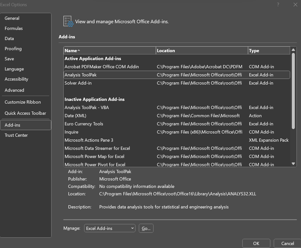
- Make sure you have activated the Excel Add-in Analysis ToolPak.
Go to the Data tab.. It is active if you have an icon with Data Analysis in the header.

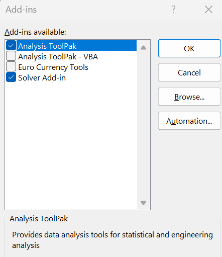
If it is not there. Go to File>Options>Add-ins and click Go on Manage Excel Add-ins
Tick the box for Analysis ToolPak and Solver Add-in (we will use it later on) and click OK.
Descriptive statistics
Go to the sheet data sample. This is the first three columns from the breast-cancer data set. We will use this to illustrate the functions for summary statistics.
Go to the sheet sample summary. Here we show what you get out from running Data>Data Analysis>Descriptive Statistics. Try this!
We also show examples of functions to derive descriptive statistics from a data sample.
Tip
Click on the name of the function in the editor to open it’s help text

- Calculate the three summary statistics described in the green area of the sheet.
The third quartile in the sample, P75, should be 15.78
The 5% quantile (or 5th percentile), P05, should be 9.52
The coefficient of variation is the ratio between the sample standard deviation and the sample mean, and should be 25%
Tip
Solutions are found at the end of this document - but try first!
Histogram
- Go to the sheet plot a histogram and explore the two ways to create a histogram.
Probability functions
- Go to the sheet probability functions.
Here we listed the functions available in a standard Excel. A density (PDF) and a probability (CDF) is calculated using the function ending with .DIST, but with different arguments. A quantile is calculated with the function ending with .INV. Different distributions are considered by using the name or short name before .DIST or .INV.
- Calculate the probability that a normally distributed variable with mean 14 and standard deviation 3.5 is less than 10
- Answer should be 0.127
- Find the 95% quantile in the same distribution
- Answer should be 19.8
- Calculate the probability that an exponentially distributed variable with mean 14 is less than 10
- Answer should be 0.51
Plot probability distributions
The general principle to plot a function is to create pairs of x-y values that are connected by a line.
- Go to the sheet plot probability distribution and study the plotting of the probability density function for a normal distribution with mean 14 and standard deviation 3.5.
Column A: pp-values are probabilities going from 0.01 to 0.99 - this is a trick to avoid having to create new x-values every time we change the parameters of the distribution.
Column B: the x-values are generated by calculating the quantile for each pp-value
Column C: the y-values (probability density) is calculated for each x-value
- See what happens when you change the values of the parameters mean and standard deviation (yellow cells)
Tip
The only thing you need to change are the parameters!
Linking functions to each other will save a lot of time and reduce the risk for errors when you work with excel.
Extra
If you feel you have the time or do another time:
Copy the sheet and refine the grid by using pp-values from 0.001 to 0.999.
Random sampling
- Go to the sheet random sampling.
All sample generators start with a random number between 0 and 1. This is also a sample from a uniform distribution.
Tip
Press F9 to make a new draw
- Type into cell D4 a function that generates a uniform random number in the interval 1 to 6. Hint: check out the help text for RAND
A random draw from a probability distribution can be generated by the inverse method. - Draws pp-values from a uniform distribution between 0 and 1 - Transform them into quantiles of the target distribution
The inverse method is demonstrated in cell D6 where it generates random draws from a normal distribution
In cell D8 we draw from a beta distribution
The inverse method is used for generating random values from probability distributions in Monte Carlo simulations.
Compare descriptive statistics against theoretical values
Wow - now we can generate data where we know the true value on parameters and all theoretical probabilities and quantiles, and compare with what we get when deriving descriptive statistics from the random sample.
Now we can explore the importance of large number of random numbers to gett good approximations when doing Monte Carlo simulations.
- Go to the final sheet compare
This sheet generates a random sample from a beta distribution.
A beta distribution has two parameters \(\alpha\) and \(\beta\)
The expected value of a beta distributed variable is \(\frac{\alpha}{\alpha+\beta}\)
- Compare the calculated sample average to the theoretical expected value (green cells)
We can also derive the theoretical quantile, let us say the P95.
- Compare the quantile from the sample with the quantile calculated from the inverse probability distribution function (blue cells)
- Which of them has the smallest difference? Why do you think it is like that?
Extra
If you feel you have the time or do another time:
Explore what happens with the difference between theoretical and statistical values when you increase sample size from 20 to a high number (close to 1000)?
Tip: Drag the formula in column B27 down to a row with a large number.
Solutions
Functions in Excel
QUARTILE.INC(‘data sample’!C:C,3)
PERCENTILE.INC(‘data sample’!C:C,0.05)
STDEV.S(‘data sample’!C:C)/AVERAGE(‘data sample’!C:C)*100
NORM.DIST(10,14,3.5,1)
NORM.INV(0.95,14,3.5)
EXPON.DIST(10,1/14,1)
RAND()*(6-1)+1
Functions in R
You can find a reproduction of the calculations, visualisations and simulations using R.