Chance, belief and frequency

MVEN10 Risk Assessment in Environment and Public Health

Author

Ullrika Sahlin

Exercise overview

Work in groups of 4-5

Background

Probability is a mathematical concept defined basic rules.

The basic rules of probability

Definition: The probability of an event A, denoted P(A), is a number between 0 and 1, with P(A) = 0 corresponding to A being impossible, and P(A) = 1 to A being certain.

Complement rule: P(not A) = 1 - P(A)

Addition rule:

for mutually exclusive events A, B: P(A or B) = P(A) + P(B)

for non-mutually exclusive events A, B: P(A or B) = P(A) + P(B) - P(A and B)

Multiplication rule:

for independent events A, B: P(A and B) = P(A) x P(B)

for dependent events A, B: P(A and B) = P(A|B) x P(B) where P(A|B) is the conditional probability of A given B

There are different ways to interpret and use probability, sometimes within the same assessment. In this exercise you will be exposed to probability as a

Theoretical probability: The number of outcomes favouring the event, divided by the total number of outcomes, assuming the outcomes are all equally likely.
Frequency: The proportion of times, in the long run of identical circumstances that the event occurs.
Subjective probability: A persons confidence that an event will occur, expressed as a number between 0 and 1.

Purpose

To understand common interpretations of probability and for what they are used

Content

Experiment to illustrate the frequency interpretation of probability
Theoretical probability vs Expected frequency
Subjective probability

Duration

30 minutes

Reporting

No reporting required

References

I have used examples and text from the book Teaching probability by Jenny Gage and David Spiegelhalter from 2016. Cambridge University Press.

Frequency

The experiment is setup as follows:

Assign one student to flip the symmetric coin of the type Antoninus Pius - Bronze Sestertius - Roman Empire using the virtual coin flipper on random.org
Record if the outcome is heads or tails.
Assign another student to throw a six sided dice using the virtual dice roller on random.org
Record if the outcome is a number in the range 1 to 5 or a six
Repeat N=5 times

Assign one student to record the outcomes in this frequency tree (replace N and # with numbers).

flowchart LR
  A("N") -->|heads|B("#")
  A("N") -->|tails|C("#")
  B("#") -->|1 to 5|D("#")
  B("#") -->|six|E("#")
  C("#") -->|1 to 5|F("#")
  C("#") -->|six|G("#")

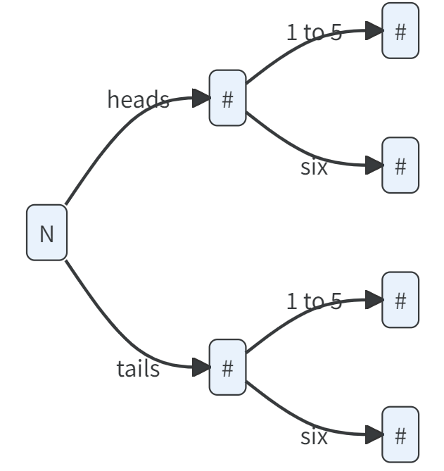
Answer the following questions:

What is the observed frequency of the event “heads followed by a six”?

Expected frequency

Is this a reliable estimate of the expected frequency? If not, what can one do to make it more reliable?
What do you expect the frequency to be if N would be a very large number?

Tip

Define the events A = “heads” and B = “six”.

Specify P(A) and P(B).

Calculate P(A and B) using the multiplication rule for two independent events.

Don’t forget to multiply by N to get the expected frequency.

Repeat the experiment with N = 100 to verify if estimates of the expected frequencies become more reliable with a larger number of observations.

Tip

You can use the prepared spreadsheet in frequency_experiment.xlsx

First you have to figure out how to expand the formulas for 100 iterations.

Chance

Now let us go back to the step where you specified the probabilities P(A) and P(B). How did you do that? One way to do it is to look at the outcome space, find the outcomes that correspond to the event and divide by the total number of outcomes.

For the coin the outcome space is “heads” and “tails”, i.e. n = 2. The event of a getting “heads” can occur in one of the outcomes, i.e. m = 1. Under the assumption that all outcomes are equally likely, the theoretical probability for “heads” is \(\frac{m}{n} = \frac{1}{2}\).

For the dice, the outcome space is 1, 2, 3, 4, 5, and 6, i.e. n = 6. The event of getting a “six” can occur in one way, i.e. m = 1. The theoretical probability for the event “six” is therefore \(\frac{1}{6}\).

Note

Notice that theoretical probabilities can only be used in balanced situations such as dice, cards, or lottery tickets where it justified to assume symmetry (equal probability) for all possible outcomes.

Relative frequency

If we divide the frequency of an event by the number of trials N, we get the relative frequency which is a good estimate of a probability for the event to occur at the next iteration of the same experiment.

Let \(m\) be the number of times the event has occurred. \(E(\frac{m}{N})=\frac{E(m)}{N}=\frac{N\cdot P(event)}{N} = P(event)\)

Relative frequencies can be used to estimate the probability for an event as long as the observations are equally likely across the full outcome space.

Make sure N is large

The more observations (i.e. larger N) the better estimate.

The more extreme event, i.e. very low or high probability of occurring, the more observations are needed.

Be very skeptical to estimates of probabilities that are either 0 and 1, when the event is possible to occur.

Belief

Take one of the thumbtacks provided in the exercise and a cup. Put the thumbtack in the cup, shake and place the cup upside down on a table without revealing the outcome.

What outcomes are possible?

Focus on the outcome that the thumbtack is having its head down with the needle pointing upwards.

Let everyone in the group state their personal probability of this event as a number between 0 and 1, where 0 means that it is impossible to occur and 1 means that it is certain to occur.

Cromwell’s rule

Probabilities 1 (“the event will definitely occur”) or 0 (“the event will definitely not occur”) should be avoided, except when applied to statements that are logically true or false.

Discuss if and why the probabilities differ.

This is an example of probability as a subjective probability that is purely a personal judgement based on available evidence and assumptions.

More evidence ought to result in smaller divergence in judgements. One way to illustrate this is to lift the cup and let everyone revise their judgement.

Do that!

Given that the evidence is revealing the outcome, the subjective probabilities held by the students in the group should now be either 1 or 0.

In risk assessment, we seldom have such full certainty as in this example. Probabilities are almost inevitably based on judgements and assumptions such as random sampling.

A general advice

Probability can be thought of as an expected frequency. Instead of saying that “the probability of the event is 0.20 (or 20%)”, you can say “out of 100 situations like this, we would expect the event to occur 20 times”.

By carefully stating the denominator (reference class), ambiguity about the meaning of probability can be avoided.

This advice applies to any of the interpretations.