Exercise 13. Daily intake equation - solutions for Monte Carlo simulations

MVEN10 Risk Assessment in Environment and Public Health

Author

Ullrika Sahlin

Problem

In excercise 12 you got the task to suggest how to set up (implement) a Monte Carlo simulation for the dose equation provided in chapter 10.8.1.

\[Dose = \frac{C \cdot IR \cdot EF}{bw}\] where

\(C\) is the concentration of the substance in the medium (mg/l)
\(IR\) is intake rate (l/day)
\(EF\) is exposure frequency (part of year; unitless), and
\(bw\) body weight (g)

\[C \sim N(0.00063,0.000063)\] \[ IR \sim N(5,05)\]

\[ EF \sim U(0.12,0.18)\]

\[ bw \sim N(25.11,2.51)\]

Here we will look at a solution in Excel and a solution in R.

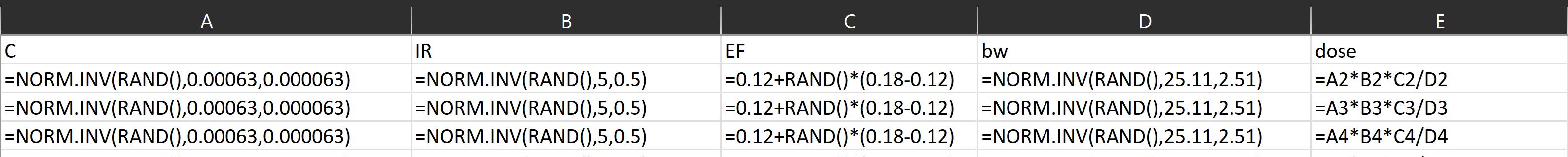
Solution for Monte Carlo simulation done in Excel

Download the file, open it and go to sheet 1.

Random numbers are generated by using the functions RAND() and NORM.INV

Solution for Monte Carlo simulation done R

Load useful packages

library(dplyr)


Attaching package: 'dplyr'

The following objects are masked from 'package:stats':

    filter, lag

The following objects are masked from 'package:base':

    intersect, setdiff, setequal, union

library(ggplot2)

Draw niter random numbers from the input distributions

niter = 10^4
df <- data.frame(
  C = rnorm(niter,0.00063,0.000063),
  IR = rnorm(niter,5,0.5),
  EF = runif(niter,min=0.12,max=0.18),
  bw = rnorm(niter,25.11,2.51)) %>%
  mutate(dose = C*IR*EF/bw)

Calculate the probability that the dose exceeds \(3 \cdot 10^-5\)

threshold = 0.00003 
mean(df$dose > threshold)

[1] 0.008

Calculate the 95th percentile for the dose

quantile(df$dose, probs = 0.95)

         95% 
2.614251e-05

Visualise the distribution of dose in a histogram

df %>% 
  ggplot(aes(x = dose)) +
  geom_histogram(binwidth = 0.000001) +
  geom_vline(xintercept=threshold,col='red')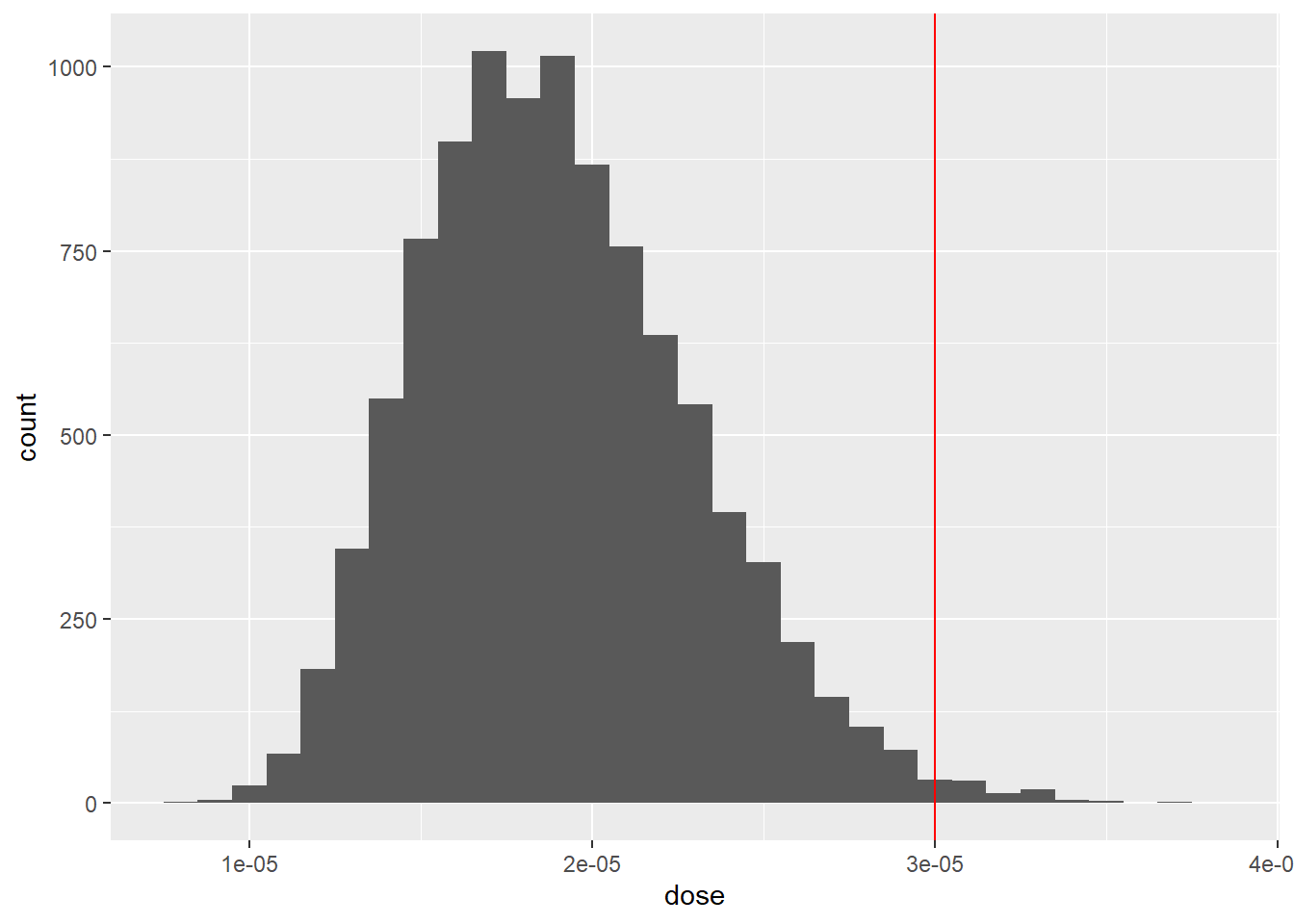

Dependencies

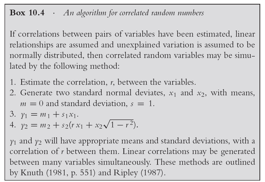
Add dependency between intake rate and body weight using the formula presented in Box 10.4 of the book where you assume a correlation of \(r = 0.9\)

For solution in Excel - study sheet 2 of the previously downloaded file

niter = 10^4
r = 0.9
x1 = rnorm(niter)
x2 = rnorm(niter)

y1 = 5 + 0.5*x1
y2 = 25.11 + 2.51*(r*x1 + x2*sqrt(1-r^2))

plot(y1,y2)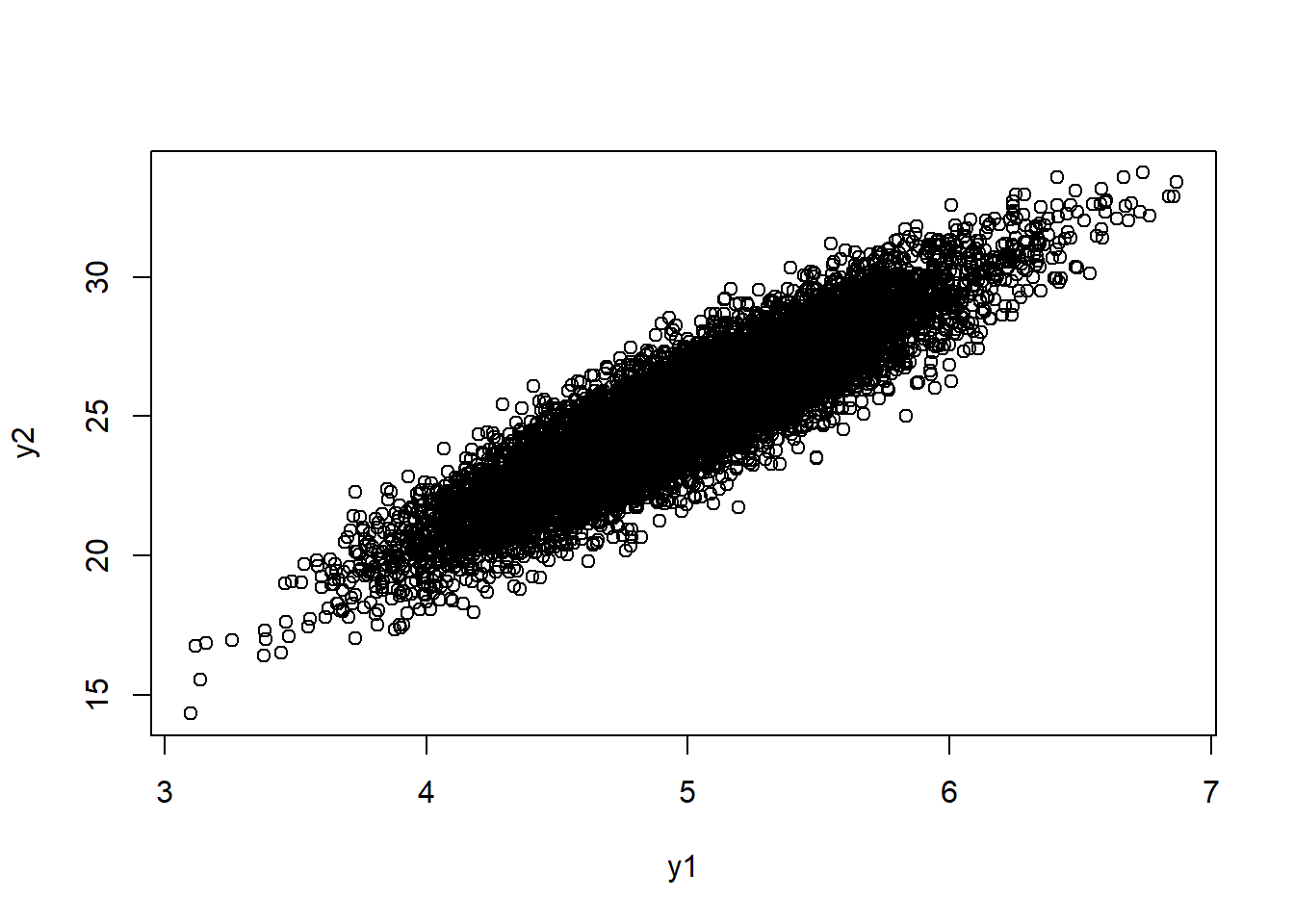

df2 <- data.frame(
  C = rnorm(niter,0.00063,0.000063),
  x1 = rnorm(niter),
  x2 = rnorm(niter),
  EF = runif(niter,min=0.12,max=0.18)) %>%
  mutate(IR = 5 + 0.5*x1) %>%
  mutate(bw = 25.11 + 2.51*(r*x1 + x2*sqrt(1-r^2))) %>%
  mutate(dose = C*IR*EF/bw)

df2 %>% 
  ggplot(aes(x = dose)) +
  geom_histogram(binwidth=0.000001) +
  geom_vline(xintercept=threshold,col='red')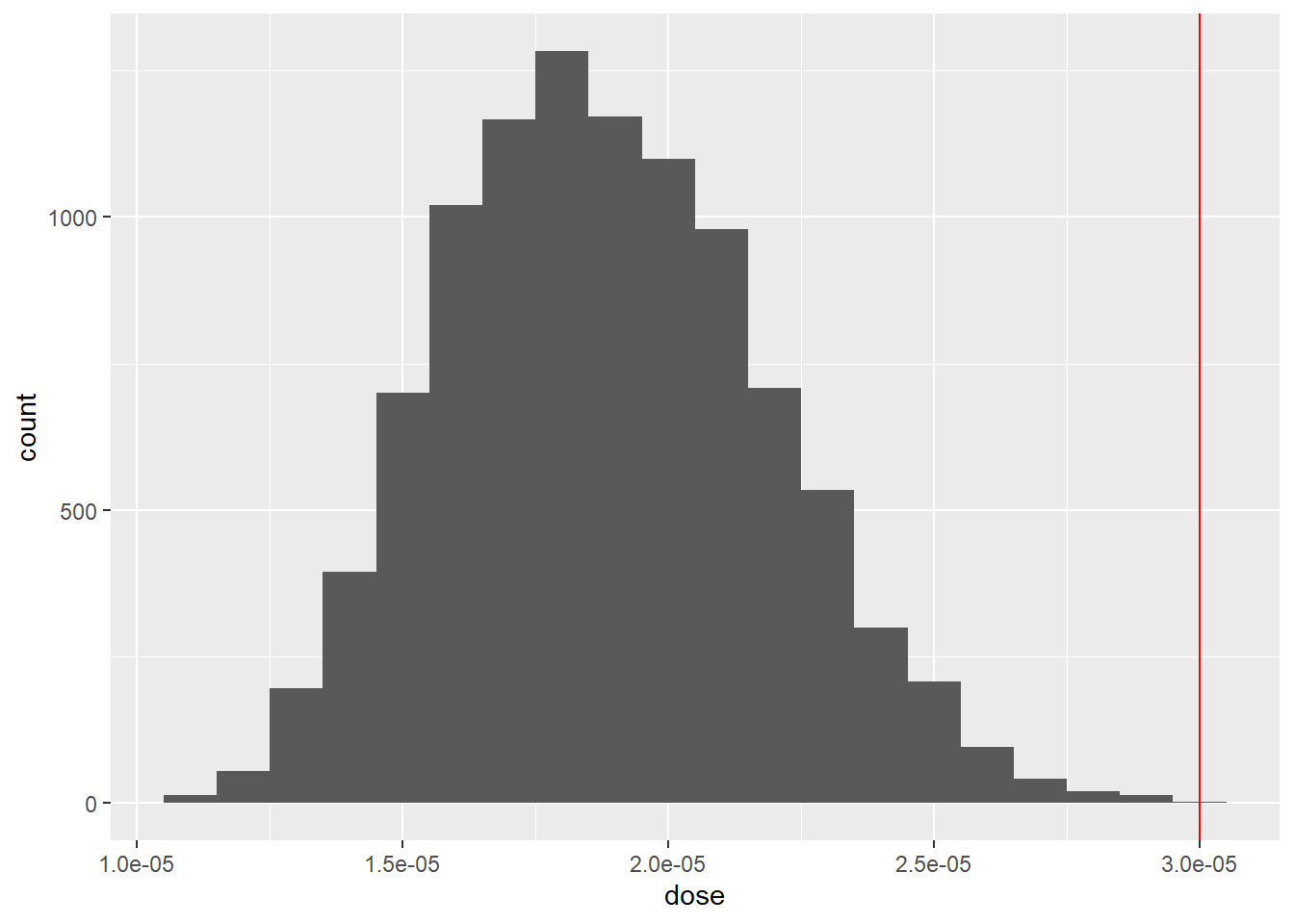

mean(df2$dose > threshold)

[1] 0

quantile(df2$dose, probs = 0.95)

        95% 
2.39784e-05