Risk classification
MVEN10 Risk Assessment in Environment and Public Health
Exercise overview
- Work in pairs or alone.
Background
A classification model is a model that assigns cases into two or more classes. Here we focus on the problem to classify breast cancers into malignant (cancerous) or benign (non cancerous).
There are two types of errors
a benign cancer is classified as positive - this is referred to as a false positive (TP)
a malignant cancer is classified as negative - this is referred to as a false negative (FN)
All four possible outcomes of applying a binary classification model can be presented in a confusion matrix
| True situation | Positive prediction | Negative prediction |
|---|---|---|
| Cancerous | True positive (TP) | False negative (FN) |
| Non cancerous | False positive (TP) | True negative (TN) |
Desirable properties of a classification model are that its performance has
High probability of correct classifications
Low probability of both type of errors
In simple terms a binary classifier consists of
an indicator (a quantity that can be a single predictor or derived from a combination of several predictors)
a cutoff for the indicator
A modeler sets the cutoff of the indicator to achieve a desired performance of the model using
a data set with known cases and values on the predictors
a rule to trade-off the two types of errors
The Receiver Operating Curve (ROC) methodology is one way to make such trade-off of a binary classifier.
Purpose
The purpose of this exercise is to
become familiar with errors from a classification model
work with a classifier using the ROC methodology
gain experience in comparing alternative classification models
to gain more R skills
Content
Load data
Build a simple classifier and calculate frequency of different types of errors
Evaluate the classifier using the ROC curve methodology
Build another classifier and compare the two models
Duration
45 minutes
Reporting
No report
References
The data set Binary Classification Prediction for type of Breast Cancer is downloaded from Kaggle
Instructions to excercise and reporting
Open an new Quarto document in R Studio cloud, save it in a folder named ex and paste in the code or modify the code following the steps in the exercise.
When you have gone through all steps, it is time to prepare a report.
Load and visualise data
Read in data
Create a new folder named data in the directory of your project on R Studio cloud.
Download the data file and save it in the the directory of your project on R Studio cloud.
- Load the data into a data frame that you name df
To do this you load two R packages. One to read in files and one to tidy your data.
To view the data fram type df (done in the code below).
library(readr)
library(tidyr)
df <- as_tibble(read_csv("../data/breast-cancer.csv"))
df
# A tibble: 569 × 32
id diagnosis radius_mean texture_mean perimeter_mean area_mean
<dbl> <chr> <dbl> <dbl> <dbl> <dbl>
1 842302 M 18.0 10.4 123. 1001
2 842517 M 20.6 17.8 133. 1326
3 84300903 M 19.7 21.2 130 1203
4 84348301 M 11.4 20.4 77.6 386.
5 84358402 M 20.3 14.3 135. 1297
6 843786 M 12.4 15.7 82.6 477.
7 844359 M 18.2 20.0 120. 1040
8 84458202 M 13.7 20.8 90.2 578.
9 844981 M 13 21.8 87.5 520.
10 84501001 M 12.5 24.0 84.0 476.
# ℹ 559 more rows
# ℹ 26 more variables: smoothness_mean <dbl>, compactness_mean <dbl>,
# concavity_mean <dbl>, `concave points_mean` <dbl>, symmetry_mean <dbl>,
# fractal_dimension_mean <dbl>, radius_se <dbl>, texture_se <dbl>,
# perimeter_se <dbl>, area_se <dbl>, smoothness_se <dbl>,
# compactness_se <dbl>, concavity_se <dbl>, `concave points_se` <dbl>,
# symmetry_se <dbl>, fractal_dimension_se <dbl>, radius_worst <dbl>, …- Narrow down the data set to include two predictors for the classifier: mean radius and mean compactness of the cancer.
The R-package dplyr has useful functions for wrangling data. The %>% is called a pipe that makes it possible to add functions to functions.
library(dplyr)
df %>% select(c(diagnosis, radius_mean, compactness_mean))
# A tibble: 569 × 3
diagnosis radius_mean compactness_mean
<chr> <dbl> <dbl>
1 M 18.0 0.278
2 M 20.6 0.0786
3 M 19.7 0.160
4 M 11.4 0.284
5 M 20.3 0.133
6 M 12.4 0.17
7 M 18.2 0.109
8 M 13.7 0.164
9 M 13 0.193
10 M 12.5 0.240
# ℹ 559 more rowsVisualise predictors
It is always good to look at data to get a feel for it. Is it continuous, categorical or discrete numbers? What is the range of values.
Since we will use the predictors to classify, it can be useful to summarise the values of the predictors after dividing the data according to the diagnosis. If it is a good predictor, we expect the data to look different between the groups.
- Visualise the predictors per diagnose group.
Below we use density graphs, which can be thought of as a smooth histogram.
library(ggplot2)
df %>% select(c(diagnosis, radius_mean, compactness_mean)) %>%
ggplot(aes(x=radius_mean, fill=diagnosis)) +
  geom_density(alpha=0.5)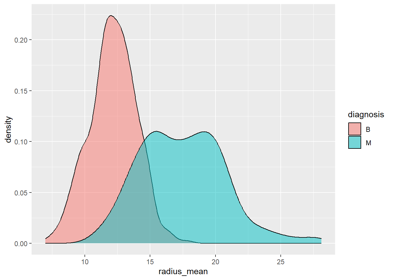
df %>% select(c(diagnosis, radius_mean, compactness_mean)) %>%
ggplot(aes(x=compactness_mean, fill=diagnosis)) +
  geom_density(alpha=0.5)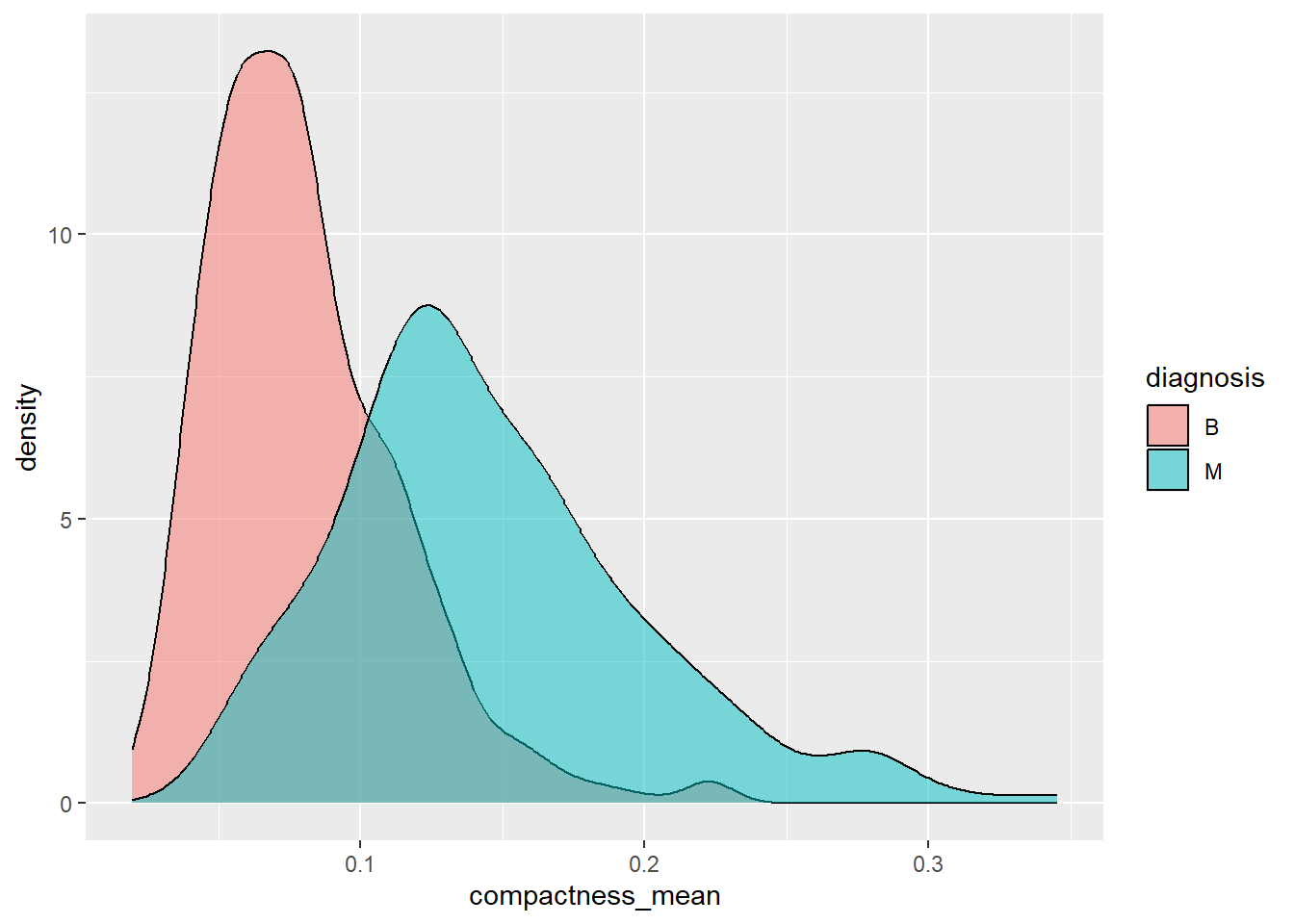
Information to put in the report
Which of the two predictors do you think is the better indicator to classify cancers into malignant or benign? Motivate your choice based on the two visualisations plots.
Include the plots in the report.
In this exercise you will build two models, one per predictor and then compare them.
Model with mean radius as predictor
- Select a cutoff of 15 for the predictor radius_mean and classify data into positive if the predictor is above the cutoff and negative if the predictor is below the cutoff. Save the predictions as pred_rad.
In the code this is done by the functions mutate and case_when.
df %>% select(c(diagnosis, radius_mean, compactness_mean)) %>%
  mutate(pred_rad=case_when(radius_mean>15 ~ "pos", .default = 'neg'))
# A tibble: 569 × 4
diagnosis radius_mean compactness_mean pred_rad
<chr> <dbl> <dbl> <chr>
1 M 18.0 0.278 pos
2 M 20.6 0.0786 pos
3 M 19.7 0.160 pos
4 M 11.4 0.284 neg
5 M 20.3 0.133 pos
6 M 12.4 0.17 neg
7 M 18.2 0.109 pos
8 M 13.7 0.164 neg
9 M 13 0.193 neg
10 M 12.5 0.240 neg
# ℹ 559 more rows- Derive the frequency of the confusion matrix for the classification model with the mean radius as predictor.
The code below selects the two variables and counts the frequency of each combination of the two variables using the function table.
Tip
To read the help text for a function type a ? followed by the name of the function in the Console. Or put your cursor on top of the function and press F1.
table(df %>% select(c(diagnosis, radius_mean, compactness_mean)) %>%
  mutate(pred_rad=case_when(radius_mean>15 ~ "pos", .default = 'neg')) %>%
  select(c(diagnosis,pred_rad)))
pred_rad
diagnosis neg pos
B 345 12
M 51 161Note that the output from table is here in the reversed order compared to the standard format of a confusion matrix. The reason is that the categories are ordered in alphabetic order.
Information to add in the report
For the binary classification model using mean radius as predictor:
What is the frequency of False positives (FP)?
What is the frequency of False negatives (FN)?
Which of these two errors do you think is worse? Motivate your answer.
Sensitivity and specificty to measure performance of a binary classifier
Sensitivity is the fraction of true positives, i.e. \(\frac{TP}{TP + FN}\) and describes the proportion of malignant cancers correctly predicted as positive.
Specificity is the fraction of true negatives, i.e. \(\frac{TN}{FP + TN}\) and describes the proportion of benign cancers correctly predicted as negative.
Information to add in the report
For the binary classification model using mean radius as predictor:
What is the frequency of True Positives (TP)?
What is the frequency of True Negatives (TN)?
What is the sensitivity and specificity?
Sensitivity and specificity measures performance of the classification model. Sensitivity and specificity should be as high as possible, but increasing one will decrease the other.
The model can be tuned towards better performance by changing the cutoff value. See for example what happens when the cutoff is changed to 11.
table(df %>% select(c(diagnosis, radius_mean, compactness_mean)) %>%
  mutate(pred_rad=case_when(radius_mean>11 ~ "pos", .default = 'neg')) %>%
  select(c(diagnosis,pred_rad)))
pred_rad
diagnosis neg pos
B 84 273
M 1 211All but one malignant cancer is classified as positive, which is good, but it comes with a cost of classifying 272 benign cancers as positive.
In other words, when changing the cutoff from 15 to 11 the
sensitivity is \(\frac{211}{211+1}=0.95\) and
specificity is \(\frac{84}{273+84}=0.24\)
The ROC curve methodology
A ROC curve is a plot of sensitivity versus 1-specificity for all values of the cutoff. It can illustrate how well the model performs and help choosing the cutoff.
- Load one of the many R-packages for ROC curve analysis.
Before loading the library you might have to install it using install.packages(“pROC”). This only needs to be done ones.
The ROC curve analysis is run using the functions roc and coords
library(pROC)Type 'citation("pROC")' for a citation.
Attaching package: 'pROC'The following objects are masked from 'package:stats':
cov, smooth, varr = roc(diagnosis ~ radius_mean, data=df)Setting levels: control = B, case = MSetting direction: controls < casescoords(r) threshold specificity sensitivity
1 -Inf 0.000000000 1.000000000
2 7.3360 0.002801120 1.000000000
3 7.7100 0.005602241 1.000000000
4 7.7445 0.008403361 1.000000000
5 7.9780 0.011204482 1.000000000
6 8.2075 0.014005602 1.000000000
7 8.3950 0.016806723 1.000000000
8 8.5840 0.019607843 1.000000000
9 8.5975 0.022408964 1.000000000
10 8.6080 0.025210084 1.000000000
11 8.6445 0.028011204 1.000000000
12 8.6985 0.030812325 1.000000000
13 8.7300 0.033613445 1.000000000
14 8.8060 0.036414566 1.000000000
15 8.8830 0.039215686 1.000000000
16 8.9190 0.042016807 1.000000000
17 8.9750 0.044817927 1.000000000
18 9.0145 0.047619048 1.000000000
19 9.0355 0.050420168 1.000000000
20 9.1075 0.053221289 1.000000000
21 9.2205 0.056022409 1.000000000
22 9.2815 0.058823529 1.000000000
23 9.3140 0.061624650 1.000000000
24 9.3650 0.064425770 1.000000000
25 9.4010 0.067226891 1.000000000
26 9.4140 0.070028011 1.000000000
27 9.4295 0.072829132 1.000000000
28 9.4505 0.075630252 1.000000000
29 9.4845 0.078431373 1.000000000
30 9.5355 0.081232493 1.000000000
31 9.5865 0.084033613 1.000000000
32 9.6365 0.086834734 1.000000000
33 9.6675 0.089635854 1.000000000
34 9.6720 0.092436975 1.000000000
35 9.6795 0.095238095 1.000000000
36 9.7015 0.098039216 1.000000000
37 9.7255 0.100840336 1.000000000
38 9.7345 0.103641457 1.000000000
39 9.7400 0.106442577 1.000000000
40 9.7485 0.112044818 1.000000000
41 9.7660 0.114845938 1.000000000
42 9.7820 0.117647059 1.000000000
43 9.8170 0.120448179 1.000000000
44 9.8615 0.123249300 1.000000000
45 9.8900 0.128851541 1.000000000
46 9.9670 0.131652661 1.000000000
47 10.0400 0.134453782 1.000000000
48 10.0650 0.137254902 1.000000000
49 10.1200 0.140056022 1.000000000
50 10.1650 0.142857143 1.000000000
51 10.1750 0.145658263 1.000000000
52 10.1900 0.148459384 1.000000000
53 10.2250 0.151260504 1.000000000
54 10.2550 0.154061625 1.000000000
55 10.2750 0.162464986 1.000000000
56 10.3050 0.165266106 1.000000000
57 10.3800 0.168067227 1.000000000
58 10.4600 0.170868347 1.000000000
59 10.4850 0.176470588 1.000000000
60 10.5000 0.182072829 1.000000000
61 10.5400 0.187675070 1.000000000
62 10.5850 0.193277311 1.000000000
63 10.6250 0.196078431 1.000000000
64 10.6550 0.198879552 1.000000000
65 10.6850 0.201680672 1.000000000
66 10.7300 0.204481793 1.000000000
67 10.7750 0.207282913 1.000000000
68 10.8100 0.212885154 1.000000000
69 10.8400 0.215686275 1.000000000
70 10.8700 0.218487395 1.000000000
71 10.8900 0.221288515 1.000000000
72 10.9050 0.224089636 1.000000000
73 10.9250 0.226890756 1.000000000
74 10.9450 0.229691877 1.000000000
75 10.9550 0.229691877 0.995283019
76 10.9650 0.232492997 0.995283019
77 11.0050 0.235294118 0.995283019
78 11.0500 0.240896359 0.995283019
79 11.0700 0.249299720 0.995283019
80 11.1050 0.252100840 0.990566038
81 11.1350 0.257703081 0.990566038
82 11.1450 0.260504202 0.990566038
83 11.1550 0.263305322 0.990566038
84 11.1800 0.266106443 0.990566038
85 11.2100 0.268907563 0.990566038
86 11.2350 0.274509804 0.990566038
87 11.2550 0.277310924 0.990566038
88 11.2650 0.282913165 0.990566038
89 11.2750 0.288515406 0.990566038
90 11.2850 0.291316527 0.990566038
91 11.2950 0.294117647 0.990566038
92 11.3050 0.296918768 0.990566038
93 11.3150 0.299719888 0.990566038
94 11.3250 0.302521008 0.990566038
95 11.3350 0.305322129 0.990566038
96 11.3500 0.310924370 0.990566038
97 11.3650 0.313725490 0.990566038
98 11.3900 0.316526611 0.990566038
99 11.4150 0.322128852 0.990566038
100 11.4250 0.322128852 0.985849057
101 11.4400 0.327731092 0.985849057
102 11.4550 0.330532213 0.985849057
103 11.4650 0.333333333 0.985849057
104 11.4800 0.336134454 0.985849057
105 11.4950 0.338935574 0.985849057
106 11.5050 0.341736695 0.985849057
107 11.5150 0.344537815 0.985849057
108 11.5300 0.350140056 0.985849057
109 11.5550 0.355742297 0.985849057
110 11.5850 0.358543417 0.985849057
111 11.6050 0.366946779 0.985849057
112 11.6150 0.369747899 0.985849057
113 11.6250 0.372549020 0.985849057
114 11.6350 0.375350140 0.985849057
115 11.6500 0.378151261 0.985849057
116 11.6650 0.380952381 0.985849057
117 11.6750 0.383753501 0.985849057
118 11.6850 0.386554622 0.985849057
119 11.6950 0.389355742 0.985849057
120 11.7050 0.392156863 0.985849057
121 11.7250 0.400560224 0.985849057
122 11.7450 0.406162465 0.985849057
123 11.7550 0.411764706 0.985849057
124 11.7800 0.414565826 0.981132075
125 11.8050 0.417366947 0.976415094
126 11.8250 0.420168067 0.976415094
127 11.8450 0.422969188 0.971698113
128 11.8600 0.425770308 0.971698113
129 11.8800 0.428571429 0.971698113
130 11.8950 0.436974790 0.971698113
131 11.9150 0.439775910 0.971698113
132 11.9350 0.445378151 0.971698113
133 11.9450 0.450980392 0.971698113
134 11.9700 0.453781513 0.971698113
135 11.9950 0.456582633 0.971698113
136 12.0150 0.462184874 0.971698113
137 12.0350 0.464985994 0.971698113
138 12.0450 0.467787115 0.971698113
139 12.0550 0.473389356 0.971698113
140 12.0650 0.478991597 0.971698113
141 12.0850 0.481792717 0.971698113
142 12.1300 0.484593838 0.971698113
143 12.1700 0.487394958 0.971698113
144 12.1850 0.495798319 0.971698113
145 12.1950 0.498599440 0.971698113
146 12.2050 0.501400560 0.971698113
147 12.2150 0.507002801 0.971698113
148 12.2250 0.509803922 0.971698113
149 12.2400 0.512605042 0.971698113
150 12.2600 0.518207283 0.971698113
151 12.2850 0.523809524 0.971698113
152 12.3050 0.529411765 0.971698113
153 12.3150 0.532212885 0.971698113
154 12.3300 0.535014006 0.971698113
155 12.3500 0.543417367 0.966981132
156 12.3750 0.549019608 0.966981132
157 12.3950 0.551820728 0.966981132
158 12.4100 0.554621849 0.966981132
159 12.4250 0.557422969 0.966981132
160 12.4400 0.560224090 0.966981132
161 12.4550 0.563025210 0.962264151
162 12.4650 0.568627451 0.957547170
163 12.4800 0.574229692 0.957547170
164 12.5150 0.577030812 0.957547170
165 12.5500 0.582633053 0.957547170
166 12.5700 0.585434174 0.957547170
167 12.6000 0.588235294 0.957547170
168 12.6250 0.593837535 0.957547170
169 12.6400 0.596638655 0.957547170
170 12.6600 0.599439776 0.957547170
171 12.6750 0.602240896 0.957547170
172 12.6900 0.602240896 0.952830189
173 12.7100 0.605042017 0.952830189
174 12.7350 0.610644258 0.952830189
175 12.7550 0.613445378 0.952830189
176 12.7650 0.619047619 0.952830189
177 12.7750 0.624649860 0.948113208
178 12.7900 0.627450980 0.948113208
179 12.8050 0.630252101 0.948113208
180 12.8200 0.633053221 0.948113208
181 12.8400 0.635854342 0.943396226
182 12.8550 0.638655462 0.943396226
183 12.8650 0.644257703 0.943396226
184 12.8750 0.649859944 0.943396226
185 12.8850 0.655462185 0.943396226
186 12.8950 0.663865546 0.943396226
187 12.9050 0.666666667 0.943396226
188 12.9250 0.669467787 0.943396226
189 12.9450 0.672268908 0.943396226
190 12.9550 0.675070028 0.943396226
191 12.9700 0.677871148 0.943396226
192 12.9850 0.680672269 0.943396226
193 12.9950 0.683473389 0.943396226
194 13.0050 0.689075630 0.938679245
195 13.0200 0.691876751 0.938679245
196 13.0400 0.694677871 0.938679245
197 13.0650 0.703081232 0.938679245
198 13.0950 0.705882353 0.938679245
199 13.1250 0.708683473 0.933962264
200 13.1450 0.711484594 0.933962264
201 13.1550 0.714285714 0.933962264
202 13.1650 0.717086835 0.933962264
203 13.1850 0.719887955 0.924528302
204 13.2050 0.725490196 0.924528302
205 13.2250 0.731092437 0.924528302
206 13.2550 0.733893557 0.924528302
207 13.2750 0.739495798 0.924528302
208 13.2900 0.742296919 0.919811321
209 13.3200 0.745098039 0.919811321
210 13.3550 0.747899160 0.919811321
211 13.3750 0.750700280 0.919811321
212 13.3900 0.753501401 0.919811321
213 13.4150 0.756302521 0.915094340
214 13.4350 0.756302521 0.910377358
215 13.4450 0.756302521 0.905660377
216 13.4550 0.759103641 0.905660377
217 13.4650 0.764705882 0.905660377
218 13.4750 0.767507003 0.905660377
219 13.4850 0.767507003 0.900943396
220 13.4950 0.770308123 0.900943396
221 13.5050 0.773109244 0.900943396
222 13.5200 0.775910364 0.900943396
223 13.5350 0.778711485 0.900943396
224 13.5500 0.781512605 0.900943396
225 13.5750 0.784313725 0.900943396
226 13.6000 0.789915966 0.900943396
227 13.6150 0.789915966 0.891509434
228 13.6300 0.792717087 0.891509434
229 13.6450 0.798319328 0.891509434
230 13.6550 0.801120448 0.891509434
231 13.6700 0.806722689 0.891509434
232 13.6850 0.809523810 0.891509434
233 13.6950 0.812324930 0.891509434
234 13.7050 0.815126050 0.891509434
235 13.7200 0.817927171 0.886792453
236 13.7350 0.817927171 0.882075472
237 13.7450 0.820728291 0.882075472
238 13.7600 0.823529412 0.882075472
239 13.7750 0.826330532 0.877358491
240 13.7900 0.829131653 0.877358491
241 13.8050 0.829131653 0.872641509
242 13.8150 0.829131653 0.867924528
243 13.8350 0.829131653 0.863207547
244 13.8550 0.837535014 0.863207547
245 13.8650 0.837535014 0.858490566
246 13.8750 0.843137255 0.858490566
247 13.8900 0.845938375 0.858490566
248 13.9200 0.851540616 0.858490566
249 13.9500 0.854341737 0.858490566
250 13.9700 0.854341737 0.853773585
251 14.0000 0.854341737 0.849056604
252 14.0250 0.857142857 0.849056604
253 14.0350 0.859943978 0.849056604
254 14.0450 0.862745098 0.849056604
255 14.0550 0.865546218 0.849056604
256 14.0850 0.868347339 0.849056604
257 14.1500 0.871148459 0.849056604
258 14.1950 0.871148459 0.844339623
259 14.2100 0.873949580 0.844339623
260 14.2350 0.876750700 0.839622642
261 14.2550 0.876750700 0.830188679
262 14.2650 0.882352941 0.830188679
263 14.2800 0.882352941 0.825471698
264 14.3150 0.885154062 0.825471698
265 14.3700 0.887955182 0.825471698
266 14.4050 0.890756303 0.825471698
267 14.4150 0.893557423 0.825471698
268 14.4300 0.896358543 0.820754717
269 14.4450 0.899159664 0.820754717
270 14.4600 0.899159664 0.816037736
271 14.4750 0.901960784 0.816037736
272 14.4900 0.901960784 0.811320755
273 14.5150 0.904761905 0.811320755
274 14.5350 0.910364146 0.811320755
275 14.5600 0.910364146 0.806603774
276 14.5850 0.913165266 0.801886792
277 14.5950 0.915966387 0.801886792
278 14.6050 0.915966387 0.797169811
279 14.6150 0.918767507 0.797169811
280 14.6300 0.921568627 0.797169811
281 14.6600 0.927170868 0.797169811
282 14.6850 0.927170868 0.792452830
283 14.7000 0.929971989 0.792452830
284 14.7250 0.929971989 0.787735849
285 14.7500 0.932773109 0.787735849
286 14.7700 0.935574230 0.787735849
287 14.7900 0.935574230 0.783018868
288 14.8050 0.938375350 0.783018868
289 14.8350 0.941176471 0.783018868
290 14.8650 0.943977591 0.778301887
291 14.8850 0.946778711 0.773584906
292 14.9100 0.946778711 0.768867925
293 14.9350 0.949579832 0.768867925
294 14.9550 0.952380952 0.764150943
295 14.9650 0.955182073 0.764150943
296 14.9800 0.960784314 0.764150943
297 14.9950 0.963585434 0.759433962
298 15.0200 0.966386555 0.759433962
299 15.0450 0.969187675 0.759433962
300 15.0550 0.969187675 0.754716981
301 15.0700 0.969187675 0.750000000
302 15.0900 0.969187675 0.745283019
303 15.1100 0.971988796 0.740566038
304 15.1250 0.971988796 0.735849057
305 15.1600 0.971988796 0.731132075
306 15.2050 0.974789916 0.731132075
307 15.2450 0.974789916 0.726415094
308 15.2750 0.977591036 0.726415094
309 15.2900 0.977591036 0.721698113
310 15.3100 0.977591036 0.716981132
311 15.3300 0.977591036 0.712264151
312 15.3550 0.977591036 0.707547170
313 15.4150 0.977591036 0.702830189
314 15.4750 0.977591036 0.688679245
315 15.4950 0.977591036 0.683962264
316 15.5150 0.977591036 0.679245283
317 15.5700 0.977591036 0.674528302
318 15.6350 0.977591036 0.669811321
319 15.6800 0.977591036 0.665094340
320 15.7050 0.977591036 0.660377358
321 15.7200 0.980392157 0.660377358
322 15.7400 0.983193277 0.660377358
323 15.7650 0.983193277 0.650943396
324 15.8150 0.983193277 0.641509434
325 15.9350 0.983193277 0.636792453
326 16.0250 0.983193277 0.632075472
327 16.0500 0.983193277 0.627358491
328 16.0900 0.983193277 0.622641509
329 16.1200 0.983193277 0.617924528
330 16.1350 0.983193277 0.608490566
331 16.1500 0.985994398 0.608490566
332 16.1650 0.985994398 0.603773585
333 16.2050 0.988795518 0.603773585
334 16.2450 0.988795518 0.599056604
335 16.2550 0.988795518 0.594339623
336 16.2650 0.988795518 0.589622642
337 16.2850 0.988795518 0.584905660
338 16.3250 0.991596639 0.584905660
339 16.4050 0.991596639 0.580188679
340 16.4800 0.991596639 0.575471698
341 16.5500 0.994397759 0.575471698
342 16.6250 0.994397759 0.570754717
343 16.6700 0.994397759 0.566037736
344 16.7150 0.994397759 0.561320755
345 16.7600 0.994397759 0.556603774
346 16.8100 0.994397759 0.551886792
347 16.9250 0.997198880 0.551886792
348 17.0150 0.997198880 0.547169811
349 17.0350 0.997198880 0.542452830
350 17.0550 0.997198880 0.537735849
351 17.0700 0.997198880 0.533018868
352 17.1100 0.997198880 0.528301887
353 17.1650 0.997198880 0.523584906
354 17.1950 0.997198880 0.518867925
355 17.2350 0.997198880 0.514150943
356 17.2800 0.997198880 0.509433962
357 17.2950 0.997198880 0.504716981
358 17.3250 0.997198880 0.500000000
359 17.3850 0.997198880 0.495283019
360 17.4400 0.997198880 0.490566038
361 17.4650 0.997198880 0.485849057
362 17.5050 0.997198880 0.481132075
363 17.5550 0.997198880 0.476415094
364 17.5850 0.997198880 0.471698113
365 17.6400 0.997198880 0.466981132
366 17.7150 0.997198880 0.462264151
367 17.8000 0.997198880 0.457547170
368 17.8800 1.000000000 0.457547170
369 17.9200 1.000000000 0.452830189
370 17.9400 1.000000000 0.448113208
371 17.9700 1.000000000 0.443396226
372 18.0000 1.000000000 0.433962264
373 18.0200 1.000000000 0.429245283
374 18.0400 1.000000000 0.424528302
375 18.0650 1.000000000 0.419811321
376 18.1500 1.000000000 0.415094340
377 18.2350 1.000000000 0.405660377
378 18.2800 1.000000000 0.400943396
379 18.3800 1.000000000 0.391509434
380 18.4550 1.000000000 0.386792453
381 18.4750 1.000000000 0.382075472
382 18.5500 1.000000000 0.377358491
383 18.6200 1.000000000 0.372641509
384 18.6400 1.000000000 0.367924528
385 18.6550 1.000000000 0.363207547
386 18.7150 1.000000000 0.358490566
387 18.7900 1.000000000 0.353773585
388 18.8150 1.000000000 0.349056604
389 18.8800 1.000000000 0.344339623
390 18.9700 1.000000000 0.339622642
391 19.0100 1.000000000 0.334905660
392 19.0450 1.000000000 0.330188679
393 19.0850 1.000000000 0.325471698
394 19.1300 1.000000000 0.320754717
395 19.1650 1.000000000 0.316037736
396 19.1750 1.000000000 0.311320755
397 19.1850 1.000000000 0.306603774
398 19.2000 1.000000000 0.301886792
399 19.2400 1.000000000 0.297169811
400 19.3350 1.000000000 0.292452830
401 19.4200 1.000000000 0.283018868
402 19.4450 1.000000000 0.278301887
403 19.4900 1.000000000 0.273584906
404 19.5400 1.000000000 0.264150943
405 19.5700 1.000000000 0.254716981
406 19.6350 1.000000000 0.245283019
407 19.6850 1.000000000 0.240566038
408 19.7100 1.000000000 0.235849057
409 19.7600 1.000000000 0.231132075
410 19.7950 1.000000000 0.226415094
411 19.8050 1.000000000 0.221698113
412 19.8500 1.000000000 0.216981132
413 19.9900 1.000000000 0.212264151
414 20.1100 1.000000000 0.207547170
415 20.1450 1.000000000 0.202830189
416 20.1700 1.000000000 0.198113208
417 20.1900 1.000000000 0.188679245
418 20.2300 1.000000000 0.183962264
419 20.2750 1.000000000 0.179245283
420 20.3000 1.000000000 0.174528302
421 20.3250 1.000000000 0.169811321
422 20.3900 1.000000000 0.165094340
423 20.4550 1.000000000 0.160377358
424 20.4750 1.000000000 0.155660377
425 20.4950 1.000000000 0.150943396
426 20.5300 1.000000000 0.146226415
427 20.5600 1.000000000 0.141509434
428 20.5750 1.000000000 0.136792453
429 20.5850 1.000000000 0.132075472
430 20.5950 1.000000000 0.127358491
431 20.6200 1.000000000 0.122641509
432 20.6850 1.000000000 0.117924528
433 20.8250 1.000000000 0.113207547
434 20.9300 1.000000000 0.108490566
435 21.0150 1.000000000 0.103773585
436 21.0950 1.000000000 0.099056604
437 21.1300 1.000000000 0.094339623
438 21.2650 1.000000000 0.089622642
439 21.4650 1.000000000 0.084905660
440 21.5850 1.000000000 0.080188679
441 21.6600 1.000000000 0.075471698
442 21.7300 1.000000000 0.070754717
443 21.8800 1.000000000 0.066037736
444 22.1400 1.000000000 0.061320755
445 22.6800 1.000000000 0.056603774
446 23.1500 1.000000000 0.051886792
447 23.2400 1.000000000 0.047169811
448 23.2800 1.000000000 0.042452830
449 23.4000 1.000000000 0.037735849
450 23.8800 1.000000000 0.033018868
451 24.4400 1.000000000 0.028301887
452 24.9250 1.000000000 0.023584906
453 25.4750 1.000000000 0.018867925
454 26.4750 1.000000000 0.014150943
455 27.3200 1.000000000 0.009433962
456 27.7650 1.000000000 0.004716981
457 Inf 1.000000000 0.000000000- Plot the ROC curve
The code plots sensitivity against specificity (on reversed axis) for all possible values on the cutoff.
r %>% ggroc +
ggtitle("ROC curve predictor radius_mean") 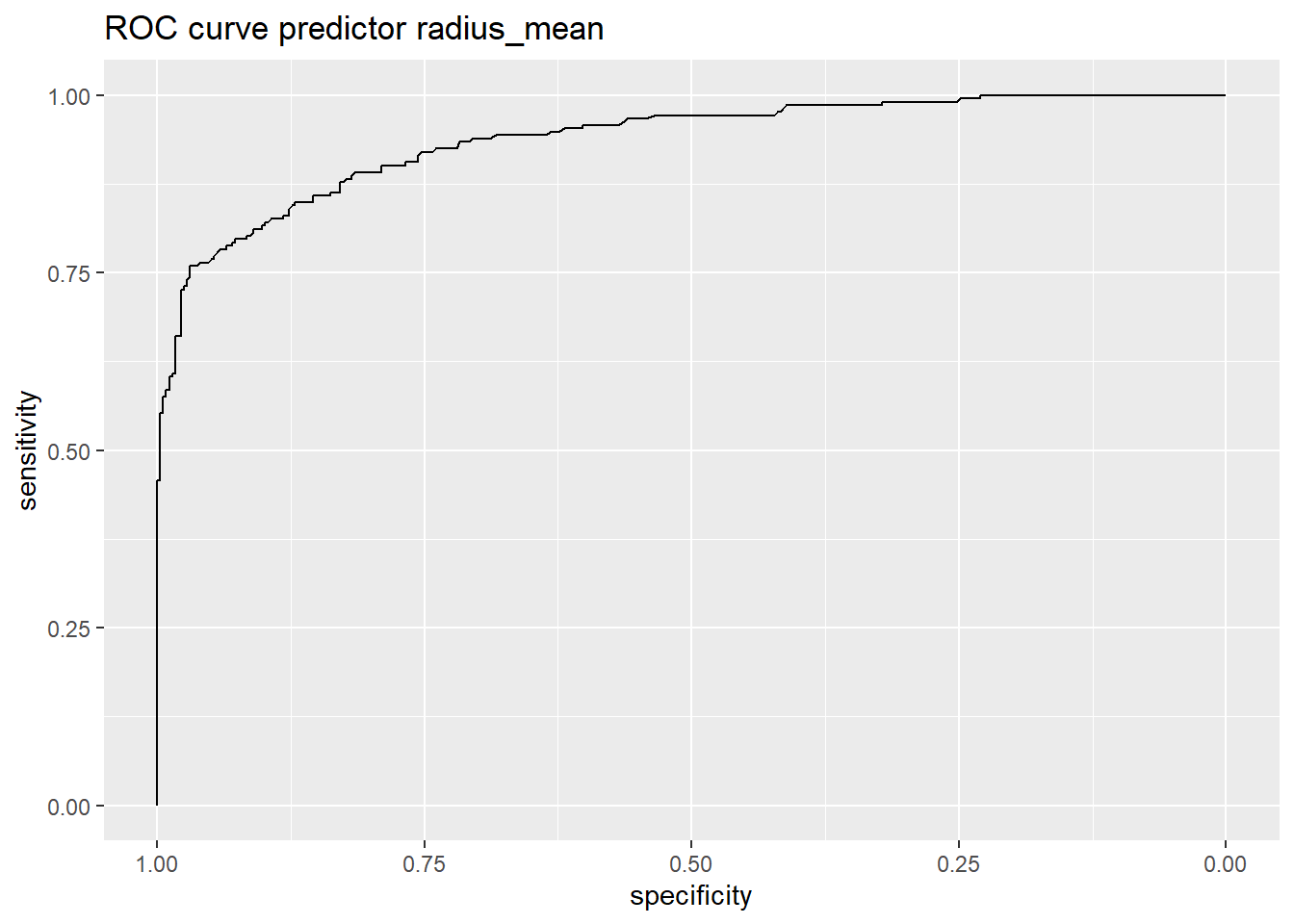
- Find a cutoff value that offers a good balance between sensitivity and specificity.
ssc = coords(r, "best", best.method = "closest.topleft")
ssc
threshold specificity sensitivity
1 14.15 0.8711485 0.8490566- Redo the plot of the ROC curve where you also add the optimal cutoff as a red point.
r %>% ggroc +
  ggtitle("ROC curve predictor radius_mean") +
  geom_point(data=ssc,aes(x=specificity,y =sensitivity),col='red')+
  annotate("text", x = ssc$specificity-0.2, y = ssc$sensitivity, label = paste0("cutoff = ", ssc$threshold))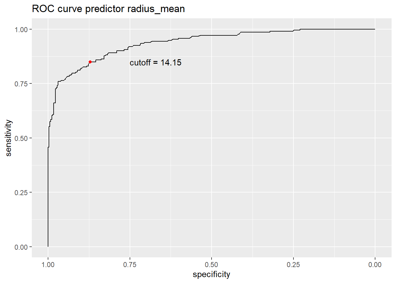
- Redo the plot and also add information about the area under the curve (AUC).
The AUC measure is useful for model comparisons, where a higher value implies a better model. A value of AUC close to 0.5 corresponds to a random guess.
r %>% ggroc +
  annotate("text", x = 0.3, y = 0.05, label = paste0("AUC = ", round(auc(r), 2))) +
  ggtitle("ROC curve predictor radius_mean") +
  geom_point(data=ssc,aes(x=specificity,y =sensitivity),col='red')+
  annotate("text", x = ssc$specificity-0.2, y = ssc$sensitivity, label = paste0("cutoff = ", ssc$threshold))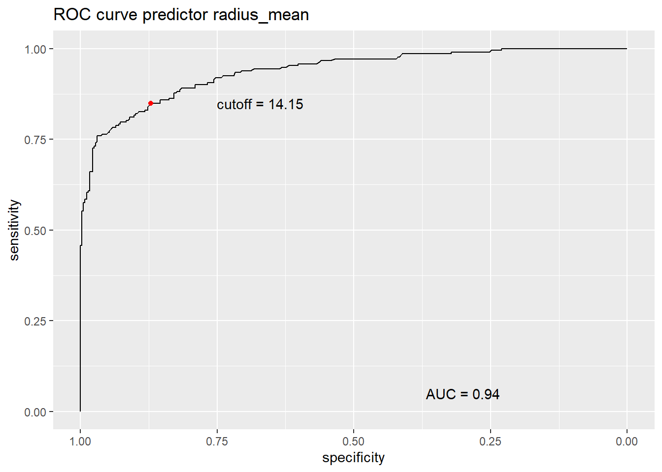
Compare classification models using the ROC curves
- Do the ROC curve analysis for the binary classification model using mean compactness as predictor.
r2 = roc(diagnosis ~ compactness_mean, data=df)Setting levels: control = B, case = MSetting direction: controls < casescoords(r2,"best", best.method = "closest.topleft") threshold specificity sensitivity
1 0.10215 0.7815126 0.8254717Which of the two models has the best performance evaluated by specificity and sensitivity?
Compare the ROC curves of the models and the area under the curves.
list(radius=r,compactness=r2) %>% ggroc +
  annotate("text", x = 0.3, y = 0.105, label = paste0("AUC radius = ", round(auc(r), 2))) +
  annotate("text", x = 0.3, y = 0.05, label = paste0("AUC compactness = ", round(auc(r2), 2))) +
  ggtitle("ROC curves")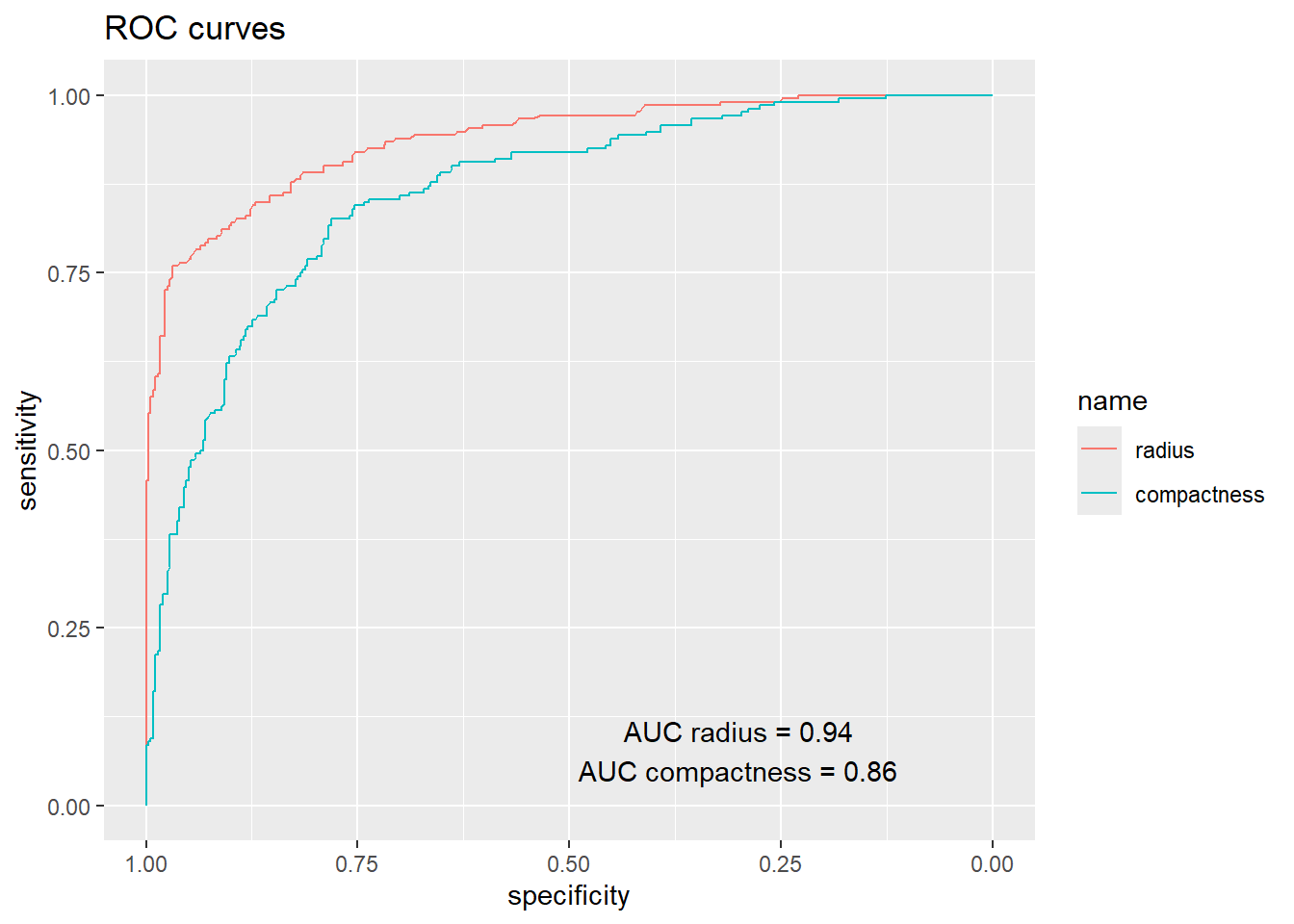
Questions
Add the graph with the two ROC curves to the project.
Which of the two binary classification models have the best performance according to the AUC measure?
Suggest three things that could be done to build a better classification model?