Solution to Exercise Coin flip in R

Author

Zheng Zhou

For comparison: Analytical solution with Beta-Binomial conjugation

# Prior: Beta(1,1), Likelihood: Binomial(100, theta)
# Posterior: Beta(1 + 55, 1 + 45) = Beta(56, 46)
analytical_mean <- 56 / (56 + 46)
analytical_sd <- sqrt((56 * 46) / ((56 + 46)^2 * (56 + 46 + 1)))

Using MCMC

library(tidyverse)

── Attaching core tidyverse packages ──────────────────────── tidyverse 2.0.0 ──
✔ dplyr     1.1.4     ✔ readr     2.1.6
✔ forcats   1.0.1     ✔ stringr   1.6.0
✔ ggplot2   4.0.1     ✔ tibble    3.3.0
✔ lubridate 1.9.4     ✔ tidyr     1.3.1
✔ purrr     1.2.0     
── Conflicts ────────────────────────────────────────── tidyverse_conflicts() ──
✖ dplyr::filter() masks stats::filter()
✖ dplyr::lag()    masks stats::lag()
ℹ Use the conflicted package (<http://conflicted.r-lib.org/>) to force all conflicts to become errors

# Metropolis Algorithm for Coin Flip
# 100 flips: 55 heads, 45 tails
# Prior: Beta(1,1)

# Define observed data
n_flips <- 100      # Total number of coin flips
n_heads <- 55       # Observed number of heads
n_tails <- 45       # Observed number of tails (or n_flips - n_heads)

# Define parameters for Metropolis algorithm
n_iterations <- 1000  # Number of MCMC iterations
starting_theta <- 0.5
proposal_sd <- 0.1

# Define the prior distribution (Beta distribution)
# Beta(1,1) is uniform over [0,1], so density is 1 for all valid thetas
prior_density <- function(theta) {
  if (theta < 0 || theta > 1) return(0)  # Prior is 0 outside [0,1]
  dbeta(theta, 1, 1)  # Beta(1,1) 
}

# Define the likelihood function (binomial probability)
likelihood_density <- function(theta) {
  # Binomial likelihood: P(data|theta) = theta^{heads} * (1-theta)^{tails}
  dbinom(n_heads, size = n_flips, prob = theta)
}

# Define the posterior density (up to proportionality constant)
posterior_density <- function(theta) {
  prior_density(theta) * likelihood(theta)  # Prior * Likelihood
}

# store the positions
chain_theta <- numeric(n_iterations)
prior_values <- numeric(n_iterations)
likelihood_values <- numeric(n_iterations)
posterior_values <- numeric(n_iterations)
acceptance_ratios <- numeric(n_iterations - 1)

# Calculate values for initial position
chain_theta[1] <- starting_theta
prior_values[1] <- prior_density(chain_theta[1])
likelihood_values[1] <- likelihood_density(chain_theta[1])
posterior_values[1] <- prior_values[1] * likelihood_values[1]  # Unnormalized posterior

# Metropolis algorithm main loop
for (i in 2:n_iterations) {
  current_theta <- chain_theta[i-1]
  
  # 1. Propose a new candidate value
  # random walk
  proposed_theta <- rnorm(1, mean = current_theta, sd = proposal_sd)
  if (proposed_theta < 0) {proposed_theta <- 1/(-proposed_theta)}
  if (proposed_theta > 1) {proposed_theta <- 1/proposed_theta}
  proposed_theta <- max(0.001, min(0.999, proposed_theta))

  # 2. Calculate acceptance ratio
  # Ratio of posterior densities: P(proposed)/P(current)
  # Calculate posterior for CURRENT state
  prior_current <- prior_density(current_theta)
  likelihood_current <- likelihood_density(current_theta)
  posterior_current <- prior_current * likelihood_current  # Unnormalized
    
  # Calculate posterior for PROPOSED state
  prior_proposed <- prior_density(proposed_theta)
  likelihood_proposed <- likelihood_density(proposed_theta)
  posterior_proposed <- prior_proposed * likelihood_proposed  # Unnormalized
  
  acceptance_ratio <- posterior_proposed / posterior_current
  acceptance_prob <- min(1, acceptance_ratio)
  
  # Store the computed values
  prior_values[i-1] <- prior_current
  likelihood_values[i-1] <- likelihood_current
  posterior_values[i-1] <- posterior_current
  acceptance_ratios[i-1] <- acceptance_prob

  # 3. Accept or reject the proposal
  if (runif(1) < acceptance_ratio) {
    chain_theta[i] <- proposed_theta
    current_theta <- proposed_theta  # Accept proposal
  } else {
    chain_theta[i] <- current_theta
  }
}

# summarize 
prior_values[n_iterations] <- prior_density(chain_theta[n_iterations])
likelihood_values[n_iterations] <- likelihood_density(chain_theta[n_iterations])
posterior_values[n_iterations] <- prior_values[n_iterations] * likelihood_values[n_iterations]

summary(posterior_values)

     Min.   1st Qu.    Median      Mean   3rd Qu.      Max. 
0.0005737 0.0394670 0.0635399 0.0562636 0.0750897 0.0799871

trace_df <- data.frame(
  iteration = 1:n_iterations,
  theta = chain_theta
)

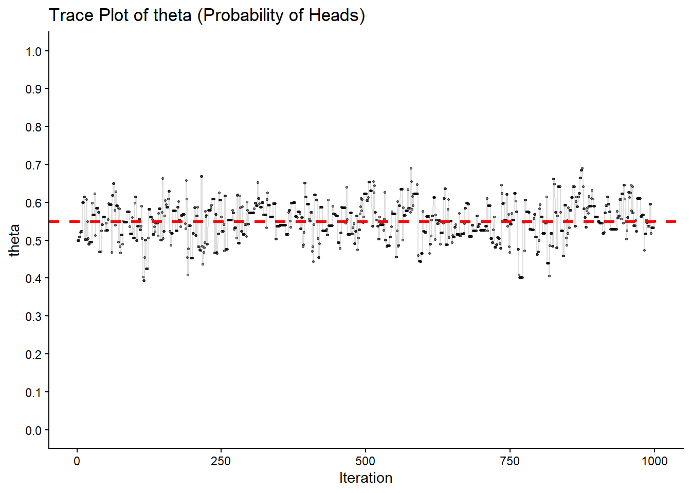
p_trace <- ggplot(trace_df, aes(x = iteration, y = theta)) +
  geom_line(alpha = 0.5, color = "gray") +
  geom_point(size = 0.5, alpha = 0.5) +
  geom_hline(yintercept = n_heads/n_flips, color = "red", linetype = "dashed", size = 1) +
  # scale_color_manual(values = c("FALSE" = "red", "TRUE" = "green"), 
  #                    na.value = "black", name = "Accepted") +
  theme_classic() +
  labs(title = "Trace Plot of theta (Probability of Heads)",
       # subtitle = paste("Red dashed line: Observed proportion =", round(n_heads/n_flips, 3)),
       x = "Iteration",
       y = "theta") +
  scale_y_continuous(limits = c(0, 1), breaks = seq(0, 1, 0.1)) +
  theme(legend.position = "bottom")

Warning: Using `size` aesthetic for lines was deprecated in ggplot2 3.4.0.
ℹ Please use `linewidth` instead.

p_trace