MCMC-sampling
BADT
Learning goals
describe what is a Markov chain monte carlo (MCMC)
describe the purpose and applicability range of MCMC
compare the strength and weakness of MCMC with other posterior estimation methods
develop a simple MCMC (complete exercise 3)
describe MCMC diagnostics
Beta-binomial conjugation
Binomial likelihood:
n Bernoulli trials with y successes and unknown probability of success \(\theta\).
\[ \text{Binomial}(n, y,\theta) \]
The prior is a beta distribution:
\[ Beta(\alpha, \beta) \]
Conjugation: the posterior distribution is also a beta distribution:
\[ Beta(\alpha + y, \beta + n - y) \]
Posterior computation
Analytical solution: conjugation often impossible
Grid approximation: possible but efficiency drops exponentialy with dimension
LaPlace approximation: assumption of multivariate normality often not applicable
Markov Chain Monte Carlo (MCMC): flexible, efficient
What is MCMC
- Markov chain
- Markov process: \(f(t+1)=g(f(t),noise)\)
- Chain
- Monte Carlo: a large number of samples can approximate the distribution
MCMC transforms the question:
FROM:
Getting the posterior distribution
TO
Getting enough representative samples from the posterior distribution
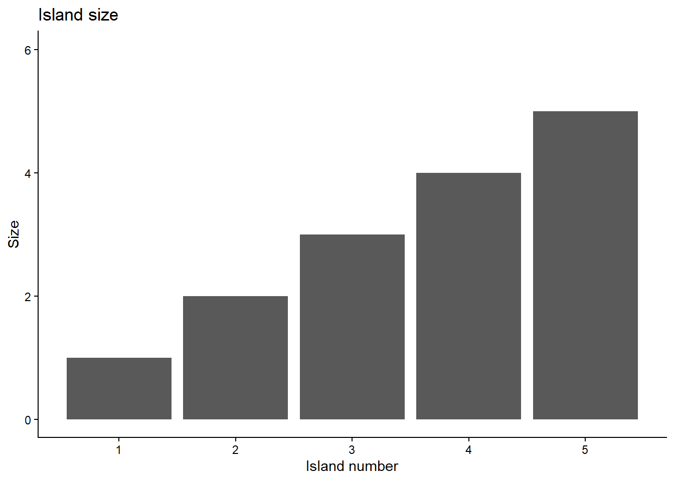
Example: Island hopping
Make a proposal.
Acceptance ratio \(p_{prop}=\frac{poposal}{current}\).
If \(p_{prop}\) > 1, move; if \(p_{prop}\)=1, stay.
If \(p_{prop}\) < 1, generate a random value k between (0,1). If \(k<p_{prop}\), then move.
repeat 1-4.
Simulate the hopping process
Number of islands (parameter values) unknown in reality.
Let’s first compute the posterior manually.
Prior: no knowledge of the islands
prior_function <- function(island) {
  return(1/num_island)  # Uniform prior
}
Likelihood: proportional to relative population of each island
likelihood_function <- function(island) {
  return(island / sum(1:num_island))  # Proportional to island size
}
Therefore, posterior = prior * likelihood / marginals
true_posterior <- sapply(1:num_island, function(i) {
  prior_function(i) * likelihood_function(i)
})
true_posterior <- true_posterior / sum(true_posterior)  # marginalize
names(true_posterior) <- paste0("Island ",1:num_island)
true_posterior
Island 1 Island 2 Island 3 Island 4 Island 5
0.06666667 0.13333333 0.20000000 0.26666667 0.33333333 Now compute the posterior with MCMC
num_iterations <- 1e3
starting_island <- 3

# store the positions
chain <- numeric(num_iterations)
prior_values <- numeric(num_iterations)
likelihood_values <- numeric(num_iterations)
posterior_values <- numeric(num_iterations)

# Calculate values for initial position
chain[1] <- starting_island
prior_values[1] <- prior_function(chain[1])
likelihood_values[1] <- likelihood_function(chain[1])
posterior_values[1] <- prior_values[1] * likelihood_values[1]  # Unnormalized posterior

# Store jump decisions for analysis
accepted <- logical(num_iterations - 1)
acceptance_ratios <- numeric(num_iterations - 1)

for(i in 2:num_iterations){
    current <- chain[i-1]

    # Propose a move: randomly jump to an adjacent island
    jump <- sample(c(-1,1), 1)
    proposed <- current + jump
    # Handle boundaries with wrap-around
    if (proposed < 1) proposed <- num_island
    if (proposed > num_island) proposed <- 1
    # random walk proposal
    # proposed <- current + rnorm(1,proposal_mean,proposal_sd)

    # compute acceptance ratio
    # current position
    prior_current <- prior_function(current)
    likelihood_current <- likelihood_function(current)
    posterior_current <- prior_current * likelihood_current  # Unnormalized

    # proposed position
    prior_proposed <- prior_function(proposed)
    likelihood_proposed <- likelihood_function(proposed)
    posterior_proposed <- prior_proposed * likelihood_proposed  # Unnormalized

    acceptance_ratio <- posterior_proposed / posterior_current
    acceptance_prob <- min(1, acceptance_ratio)

    # Store the computed values
    prior_values[i-1] <- prior_current
    likelihood_values[i-1] <- likelihood_current
    posterior_values[i-1] <- posterior_current
    acceptance_ratios[i-1] <- acceptance_prob

    # decide the jump
    if (runif(1) < acceptance_prob) {
      chain[i] <- proposed
      accepted[i-1] <- TRUE
    } else {
      chain[i] <- current
      accepted[i-1] <- FALSE
    }
}
Now summarize the results from MCMC
prior_values[num_iterations] <- prior_function(chain[num_iterations])
likelihood_values[num_iterations] <- likelihood_function(chain[num_iterations])
posterior_values[num_iterations] <- prior_values[num_iterations] * likelihood_values[num_iterations]

# Calculate empirical frequencies from MCMC samples
mcmc_freq <- table(chain) / num_iterations
mcmc_df <- data.frame(
  island = 1:num_island,
  mcmc_prob = as.numeric(mcmc_freq),
  true_posterior = true_posterior
)
mcmc_df
island mcmc_prob true_posterior
Island 1 1 0.082 0.06666667
Island 2 2 0.138 0.13333333
Island 3 3 0.176 0.20000000
Island 4 4 0.268 0.26666667
Island 5 5 0.336 0.33333333Trace the move
# Trace plot with acceptance indicators
trace_df <- data.frame(
  iteration = 1:num_iterations,
  island = chain,
  accepted = c(NA, accepted),
  posterior = posterior_values
)
p_trace <- ggplot(trace_df, aes(x = iteration, y = island)) +
  geom_line(alpha = 0.5) +
  geom_point(aes( size = posterior), alpha = 0.7) +
  # scale_color_manual(values = c("FALSE" = "red", "TRUE" = "green"),
  #                    na.value = "black", name = "Accepted") +
  scale_size_continuous(name = "Posterior", range = c(1, 3)) +
  scale_y_continuous(breaks = 1:num_island, limits = c(1, num_island)) +
  theme_classic() +
  labs(title = "Trace Plot",
       subtitle = "Point size proportional to posterior probability",
       x = "Iteration",
       y = "Island Number")
p_trace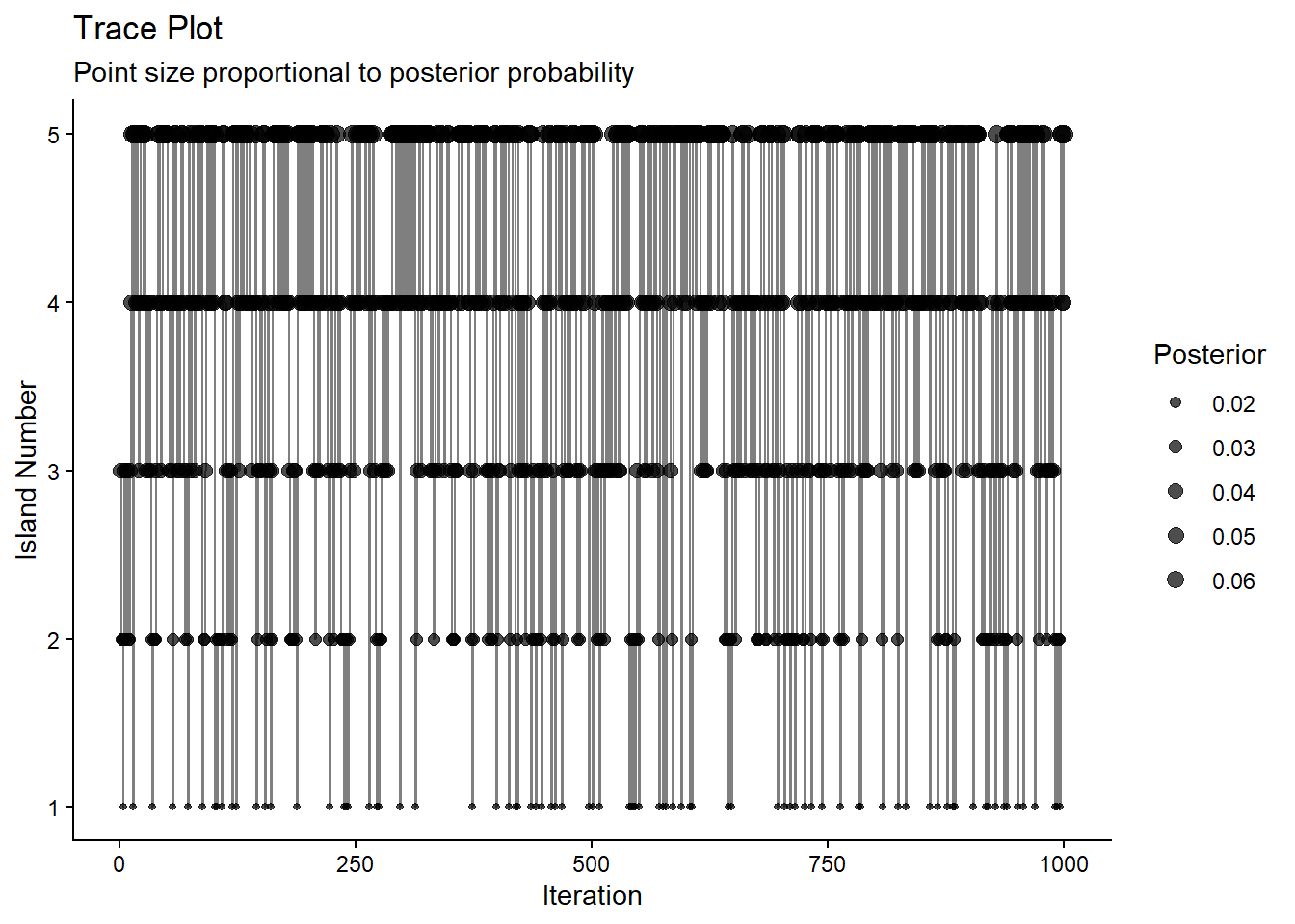
Summary of hopping
When repeated enough times, frequency on any island matches the relative population of the island.
Three critical things:
known your position and adjacent options
making a proposal and knowing the population of the proposal
knowing the population of the current, to calculate the acceptance ratio \(p_{prop}=\frac{proposal}{current}\).
Metropolis algorithm
Island hopping is a special case, Metropolis algorithm could handle:
continuous positions
more than one dimension
complex proposals
\[ y=\beta_0 + \beta_1 x + \epsilon \]
Model:
\[ \begin{equation} \begin{split} \epsilon \sim N(0,\sigma^2) \\ y \sim N(\beta_0 + \beta_1 x, \epsilon) \end{split} \end{equation} \]
\(\beta_0, \beta_1\) are parameters
Likelihood:
\[ p(Y|\beta_0,\beta_1,\epsilon,x)=\prod_i^{n} \frac{1}{\sqrt{2\pi \sigma^2}}exp(-\frac{(y-(\beta_0+\beta_1 x))^2}{2\sigma^2}) \]
Priors:
\(\beta_0 \sim N(0,5)\).
How does the island hopping analogy work here?
Metropolis algorithm
Start with an arbitrary initial value of the parameter, and denote it \(\theta_{current}\)
Randomly generate a proposed jump, \(\Delta\theta \sim N(0,\sigma^2)\) and derive the proposed parameter as \(\theta_{proposed} = \theta_{current}+\Delta\theta\).
Compute the probability of moving to the proposed value as \[\begin{split} & \\ p_{move}=min\left(1,\frac{f(\theta_{proposed}|y)}{f(\theta_{current}|y)}\right) =& \\min\left(1,\frac{l(y|\theta_{proposed})f(\theta_{proposed})}{l(y|\theta_{current})f(\theta_{current})}\right) \end{split}\]
Accept the proposed parameter value if a random value sampled from a [0,1] uniform distribution is less than \(p_{move}\)
Repeat steps 1 to 3 until a sufficiently representative sample of the posterior has been generated.
Throw away a burn-in period of the sampling and keep the part where the algorithm has converged.
The Metropolis algorithm (is a type of importance sampling) which can be combined with ways to generate proposals make the sampling more efficient, including Gibbs sampling and Hamiltonian Markov Chain (HMC).
MCMC diagnostics
Before accepting MCMC results, how good they are?
Trace plot: biased by the arbitrary starting value? fully explore the posterior range?
Rhat/ Gelman-Rubins statistics: convergence of multiple chains, also shown in the trace plot
Effective sample size: measures chain accuracy- how many independent sampling steps for the chain to approximate the posterior
Autocorrelation: also shows chain accuracy- strong correlation between steps that are one or two steps apart breaks Markov process
Read the Bayes rule book chapter 6.3 and DBDA chapter 7.5 for technical details and examples.