MCMC sampling software
Gibbs sampling and BUGS
Strength: Simple coding and similar to basic Metropolis algorithm
Weakness: Really random walks, poor at dealing with complex problems
Hamilton MC and stan
Strength: Uses gradient information to explore high-dimensional, correlated parameter space more efficiently
Weakness: Requires more coding efforts
Stan ecosystem
sampler: rstan, cmdstanr, CmdStanPy, PyMC
high-level utility package: rstanarm, brms, PyStan, bambi and more
Getting start with Stan
Installation
If you Use R : install cmdstanr
If you Use python : install cmdstanPy
install appropriate C++ toolchain based on your IDE: for R and for python
install compiler for your IDE
install utility package if desire
Once done, run an example model to check the compiler
The beta-binomial example in stan
This is cmdstanr version 0.9.0
- CmdStanR documentation and vignettes: mc-stan.org/cmdstanr
- CmdStan path: C:/Users/ekol-usa/.cmdstan/cmdstan-2.38.0
- CmdStan version: 2.38.0
<- file.path (cmdstan_path (), "examples" , "bernoulli" , "bernoulli.stan" )<- cmdstan_model (file)# names correspond to the data block in the Stan program <- list (N = 10 , y = c (0 ,1 ,0 ,0 ,0 ,0 ,0 ,0 ,0 ,1 ))# call out the stan script $ print ()
data {
  int<lower=0> N;
  array[N] int<lower=0, upper=1> y;
}
parameters {
  real<lower=0, upper=1> theta;
}
model {
  theta ~ beta(1, 1); // uniform prior on interval 0,1
  y ~ bernoulli(theta);
}
Sampling
<- mod$ sample (data = data_list,seed = 123 ,chains = 4
Running MCMC with 4 sequential chains...

Chain 1 Iteration:    1 / 2000 [  0%]  (Warmup)
Chain 1 Iteration:  100 / 2000 [  5%]  (Warmup)
Chain 1 Iteration:  200 / 2000 [ 10%]  (Warmup)
Chain 1 Iteration:  300 / 2000 [ 15%]  (Warmup)
Chain 1 Iteration:  400 / 2000 [ 20%]  (Warmup)
Chain 1 Iteration:  500 / 2000 [ 25%]  (Warmup)
Chain 1 Iteration:  600 / 2000 [ 30%]  (Warmup)
Chain 1 Iteration:  700 / 2000 [ 35%]  (Warmup)
Chain 1 Iteration:  800 / 2000 [ 40%]  (Warmup)
Chain 1 Iteration:  900 / 2000 [ 45%]  (Warmup)
Chain 1 Iteration: 1000 / 2000 [ 50%]  (Warmup)
Chain 1 Iteration: 1001 / 2000 [ 50%]  (Sampling)
Chain 1 Iteration: 1100 / 2000 [ 55%]  (Sampling)
Chain 1 Iteration: 1200 / 2000 [ 60%]  (Sampling)
Chain 1 Iteration: 1300 / 2000 [ 65%]  (Sampling)
Chain 1 Iteration: 1400 / 2000 [ 70%]  (Sampling)
Chain 1 Iteration: 1500 / 2000 [ 75%]  (Sampling)
Chain 1 Iteration: 1600 / 2000 [ 80%]  (Sampling)
Chain 1 Iteration: 1700 / 2000 [ 85%]  (Sampling)
Chain 1 Iteration: 1800 / 2000 [ 90%]  (Sampling)
Chain 1 Iteration: 1900 / 2000 [ 95%]  (Sampling)
Chain 1 Iteration: 2000 / 2000 [100%]  (Sampling)
Chain 1 finished in 0.0 seconds.
Chain 2 Iteration:    1 / 2000 [  0%]  (Warmup)
Chain 2 Iteration:  100 / 2000 [  5%]  (Warmup)
Chain 2 Iteration:  200 / 2000 [ 10%]  (Warmup)
Chain 2 Iteration:  300 / 2000 [ 15%]  (Warmup)
Chain 2 Iteration:  400 / 2000 [ 20%]  (Warmup)
Chain 2 Iteration:  500 / 2000 [ 25%]  (Warmup)
Chain 2 Iteration:  600 / 2000 [ 30%]  (Warmup)
Chain 2 Iteration:  700 / 2000 [ 35%]  (Warmup)
Chain 2 Iteration:  800 / 2000 [ 40%]  (Warmup)
Chain 2 Iteration:  900 / 2000 [ 45%]  (Warmup)
Chain 2 Iteration: 1000 / 2000 [ 50%]  (Warmup)
Chain 2 Iteration: 1001 / 2000 [ 50%]  (Sampling)
Chain 2 Iteration: 1100 / 2000 [ 55%]  (Sampling)
Chain 2 Iteration: 1200 / 2000 [ 60%]  (Sampling)
Chain 2 Iteration: 1300 / 2000 [ 65%]  (Sampling)
Chain 2 Iteration: 1400 / 2000 [ 70%]  (Sampling)
Chain 2 Iteration: 1500 / 2000 [ 75%]  (Sampling)
Chain 2 Iteration: 1600 / 2000 [ 80%]  (Sampling)
Chain 2 Iteration: 1700 / 2000 [ 85%]  (Sampling)
Chain 2 Iteration: 1800 / 2000 [ 90%]  (Sampling)
Chain 2 Iteration: 1900 / 2000 [ 95%]  (Sampling)
Chain 2 Iteration: 2000 / 2000 [100%]  (Sampling)
Chain 2 finished in 0.0 seconds.
Chain 3 Iteration:    1 / 2000 [  0%]  (Warmup)
Chain 3 Iteration:  100 / 2000 [  5%]  (Warmup)
Chain 3 Iteration:  200 / 2000 [ 10%]  (Warmup)
Chain 3 Iteration:  300 / 2000 [ 15%]  (Warmup)
Chain 3 Iteration:  400 / 2000 [ 20%]  (Warmup)
Chain 3 Iteration:  500 / 2000 [ 25%]  (Warmup)
Chain 3 Iteration:  600 / 2000 [ 30%]  (Warmup)
Chain 3 Iteration:  700 / 2000 [ 35%]  (Warmup)
Chain 3 Iteration:  800 / 2000 [ 40%]  (Warmup)
Chain 3 Iteration:  900 / 2000 [ 45%]  (Warmup)
Chain 3 Iteration: 1000 / 2000 [ 50%]  (Warmup)
Chain 3 Iteration: 1001 / 2000 [ 50%]  (Sampling)
Chain 3 Iteration: 1100 / 2000 [ 55%]  (Sampling)
Chain 3 Iteration: 1200 / 2000 [ 60%]  (Sampling)
Chain 3 Iteration: 1300 / 2000 [ 65%]  (Sampling)
Chain 3 Iteration: 1400 / 2000 [ 70%]  (Sampling)
Chain 3 Iteration: 1500 / 2000 [ 75%]  (Sampling)
Chain 3 Iteration: 1600 / 2000 [ 80%]  (Sampling)
Chain 3 Iteration: 1700 / 2000 [ 85%]  (Sampling)
Chain 3 Iteration: 1800 / 2000 [ 90%]  (Sampling)
Chain 3 Iteration: 1900 / 2000 [ 95%]  (Sampling)
Chain 3 Iteration: 2000 / 2000 [100%]  (Sampling)
Chain 3 finished in 0.0 seconds.
Chain 4 Iteration:    1 / 2000 [  0%]  (Warmup)
Chain 4 Iteration:  100 / 2000 [  5%]  (Warmup)
Chain 4 Iteration:  200 / 2000 [ 10%]  (Warmup)
Chain 4 Iteration:  300 / 2000 [ 15%]  (Warmup)
Chain 4 Iteration:  400 / 2000 [ 20%]  (Warmup)
Chain 4 Iteration:  500 / 2000 [ 25%]  (Warmup)
Chain 4 Iteration:  600 / 2000 [ 30%]  (Warmup)
Chain 4 Iteration:  700 / 2000 [ 35%]  (Warmup)
Chain 4 Iteration:  800 / 2000 [ 40%]  (Warmup)
Chain 4 Iteration:  900 / 2000 [ 45%]  (Warmup)
Chain 4 Iteration: 1000 / 2000 [ 50%]  (Warmup)
Chain 4 Iteration: 1001 / 2000 [ 50%]  (Sampling)
Chain 4 Iteration: 1100 / 2000 [ 55%]  (Sampling)
Chain 4 Iteration: 1200 / 2000 [ 60%]  (Sampling)
Chain 4 Iteration: 1300 / 2000 [ 65%]  (Sampling)
Chain 4 Iteration: 1400 / 2000 [ 70%]  (Sampling)
Chain 4 Iteration: 1500 / 2000 [ 75%]  (Sampling)
Chain 4 Iteration: 1600 / 2000 [ 80%]  (Sampling)
Chain 4 Iteration: 1700 / 2000 [ 85%]  (Sampling)
Chain 4 Iteration: 1800 / 2000 [ 90%]  (Sampling)
Chain 4 Iteration: 1900 / 2000 [ 95%]  (Sampling)
Chain 4 Iteration: 2000 / 2000 [100%]  (Sampling)
Chain 4 finished in 0.0 seconds.

All 4 chains finished successfully.
Mean chain execution time: 0.0 seconds.
Total execution time: 0.7 seconds.
Extract model diagnostics
# install.package(c("bayesplot","tidyverse")) library (bayesplot)
This is bayesplot version 1.15.0
- Online documentation and vignettes at mc-stan.org/bayesplot
- bayesplot theme set to bayesplot::theme_default()
* Does _not_ affect other ggplot2 plots
* See ?bayesplot_theme_set for details on theme setting
── Attaching core tidyverse packages ──────────────────────── tidyverse 2.0.0 ──
✔ dplyr     1.1.4     ✔ readr     2.1.6
✔ forcats   1.0.1     ✔ stringr   1.6.0
✔ ggplot2   4.0.1     ✔ tibble    3.3.0
✔ lubridate 1.9.4     ✔ tidyr     1.3.1
✔ purrr     1.2.0
── Conflicts ────────────────────────────────────────── tidyverse_conflicts() ──
✖ dplyr::filter() masks stats::filter()
✖ dplyr::lag()    masks stats::lag()
ℹ Use the conflicted package (<http://conflicted.r-lib.org/>) to force all conflicts to become errors
Check rhat and effective sample size:
# all parameters $ summary ()
# A tibble: 2 × 10
  variable   mean median    sd   mad      q5    q95  rhat ess_bulk ess_tail
  <chr>     <dbl>  <dbl> <dbl> <dbl>   <dbl>  <dbl> <dbl>    <dbl>    <dbl>
1 lp__     -7.27  -6.99  0.750 0.323 -8.74   -6.75   1.00    1931.    2287.
2 theta     0.252  0.239 0.120 0.122  0.0806  0.477  1.00    1368.    1664.
Rhat should be as close to 1 as possible
ESS: ideally number of sampling steps from all chains
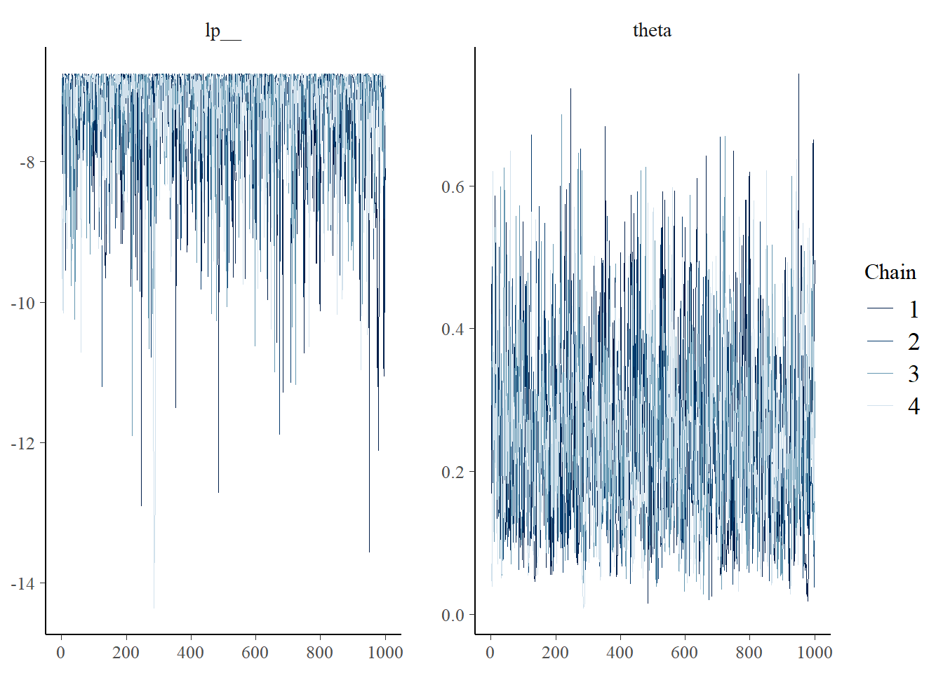
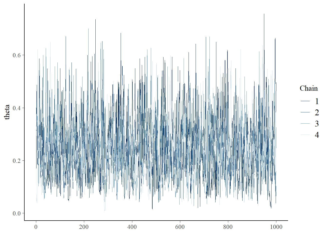
Traceplot:
# all parameters mcmc_trace (fit$ draws ())# specific parameter mcmc_trace (fit$ draws ("theta" ))
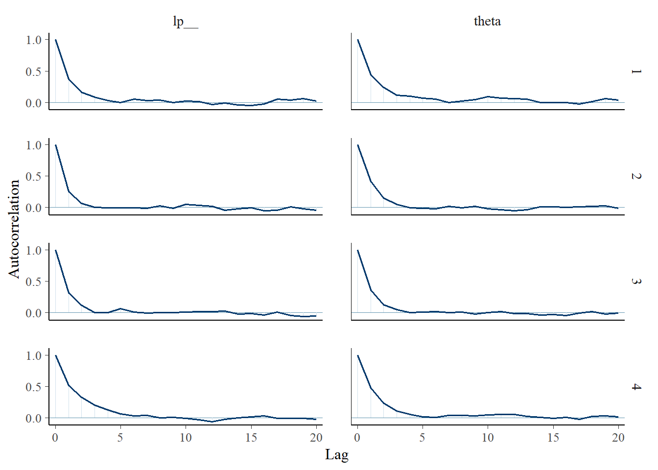
Autocorrelation:
# all parameters mcmc_acf (fit$ draws ())
When something goes wrong, check this